[Avg. reading time: 0 minutes]

[Avg. reading time: 0 minutes]
Disclaimer


[Avg. reading time: 4 minutes]
Required Tools
-
CLI
-
Python (3.11 to 3.13)
-
Python Dependency Manager (choose one)
-
Code Editor
-
VSCode Extension
-
Container Engine
Free Cloud Services
| Tool | Purpose | Link |
|---|---|---|
| Databricks Free Edition | ML & Ops | Free Signup |
| Chroma | Free Vector DB | ChromaDB |
#tools #databricks #python #git
[Avg. reading time: 2 minutes]
MLOps & AI Overview
- MLOps & AI Overview
[Avg. reading time: 3 minutes]
Introduction
AI/ML are no longer just research topics - they drive industry, innovation, and jobs.
GenAI has shifted expectations: businesses want faster solutions with production-grade reliability.
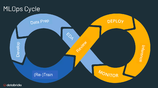
MLOps ensures ideas → working models → deployed systems.
Evolution of the Field
2010s: Big Data + early ML adoption (scikit-learn, Spark MLlib).
2015-2022: Deep learning boom (Neural Networks, NLP with BERT).
2022: Generative AI (GPT, diffusion models).
MLOps is critical for scaling, governance, monitoring.
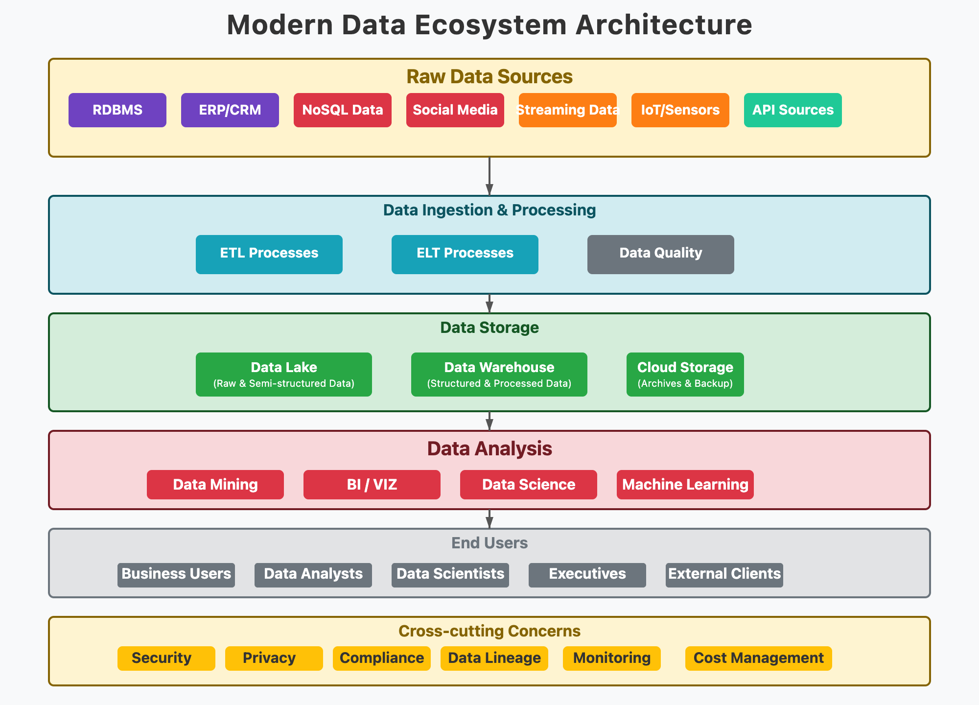
Where MLOps Fits in the Data/AI Journey
MLOps is part of all of this.
Without MLOps, many models stay as “academic projects.”
Today’s hiring market looks for hybrid skills (data + ML + cloud + ops).
Course Positioning
Not too heavy on topics covered in other courses such as ML algorithms or NLP or Deep Learning or LLM.
This course is heavy on CICD - MLOps, Pipelines, versioning, monitoring, cloud platforms and related toolsets.
Course Focus = Industry Readiness
[Avg. reading time: 0 minutes]
AI then and now

#MachineLearning #ArtificialIntelligence
[Avg. reading time: 1 minute]
Expert Systems
Early AI systems (1970s–1990s)
Rule-based: encode human expert knowledge as if-then rules.
Precursor to modern ML, focused on symbolic reasoning rather than data-driven learning.
Pros
- Transparent and explainable (rules are visible).
- Effective in narrow, well-defined domains.
Cons
- Knowledge engineering is labor-intensive.
- Doesn’t scale well as rules explode.
- Cannot adapt automatically from new data.
[Avg. reading time: 3 minutes]
Fuzzy Logic
Logic that allows degrees of truth (not just True/False). Models uncertainty with values between 0 and 1.
graph TD
    A["Is it Cold?"] --> B["Crisp Logic<br/>Yes = 1<br/>No = 0"]
    A --> C["Fuzzy Logic<br/>Maybe Cold = 0.3<br/>Not really cold = 0.7"]
Useful in control systems and decision-making under vagueness.
Still used in various use cases to find out similarity like New Jersey similar to Jersey.
Pros
- Handles imprecise, uncertain, or linguistic data (“high temperature”, “low risk”).
- Good for rule-based control.
Cons
- Not data-driven → rules must be defined manually.
- Limited learning ability compared to ML.
Use Cases
- Washing machines that adjust cycles based on “fuzziness” of dirt level.
- Air conditioning systems adapting to “comfort level”.
- Automotive control (braking, transmission).
- Risk assessment systems.
[Avg. reading time: 3 minutes]
Machine Learning
A subset of AI where systems learn patterns from data and make predictions or decisions without being explicitly programmed.
-
One of the core pillars of AI.
-
Between traditional rule-based systems (Expert Systems) and modern Deep Learning/GenAI.
-
Provides the foundation for many practical AI applications used in industry today.
Pros
- Automates decision-making at scale.
- Flexible: can be applied to structured and unstructured data.
- Improves with more data and better features.
Cons
- Requires labeled data (for supervised learning).
- Models can overfit or underfit if not designed carefully.
- Often seen as a “black box” with limited interpretability.
Use Cases
- Fraud detection in finance.
- Customer churn prediction in telecom/retail.
- Demand forecasting in supply chain.
- Email spam filtering.
- Customer segmentation for targeted marketing.
- Market basket analysis (“people who buy X also buy Y”).
- Anomaly detection in cybersecurity and IoT.
#Supervised #Unsupervised #classification #regression
[Avg. reading time: 3 minutes]
Generative AI
A class of AI that can create new content (text, code, images, video, music) rather than just predicting outcomes.
Powered by foundation models like GPT, Stable Diffusion, etc.
-
Builds on Deep Learning + NLP + multimodal modeling.
-
Represents the shift from discriminative models (predicting) to generative models (creating).
Pros
- Enables creativity and automation at scale.
- Reduces time to draft, design, or brainstorm.
Cons
- Can hallucinate false information.
- High computational cost and environmental footprint.
- Raises copyright, ethics, and bias concerns.
Use Cases
- Text: AI writing assistants, code copilots.
- Image/video: marketing content generation, design prototyping.
- Data: generating synthetic data for ML training.
- Education: personalized learning materials and quizzes.
Key differences
| Traditional ML | Generative AI |
|---|---|
| Predicts outcome from features | Produces new content |
| Needs task-specific data | Pretrained on massive corpora |
| Optimized for accuracy | Optimized for creativity, coherence |
| Example: Predict churn | Example: Generate flying pigs/elephant |
[Avg. reading time: 4 minutes]
Reinforcement Learning
RLHF (Reinforcement Learning Human Feedback)
Its like humans learning todo and not todo.
A learning paradigm where an agent interacts with an environment, takes actions, and learns from reward signals.
Instead of labeled data, it uses trial-and-error feedback.
Complements supervised/unsupervised learning.
Strongly linked to decision-making and control tasks.
Example: YT recommends a video, if you watch it system understands that, if you choose don’t show this system reacts to that.
Here the agent is YT recommendation engine, action: user watching or ignoring the video. Rewards like/share or not-interested.
Pros
- Handles complex sequential decisions.
- Can learn optimal strategies without explicit rules.
- Mimics human/animal learning.
Cons
- Data and compute intensive.
- Reward design is tricky.
- Training can be unstable.
Use Cases
- Game AI: AlphaGo defeating world champions.
- Robotics: teaching robots to walk, grasp, or navigate.
- Finance: algorithmic trading strategies.
- Dynamic pricing in e-commerce.
flowchart TD
    A[Prompt] --> B[Base LLM generates multiple responses]
    B --> C[Human labelers rank responses]
    C --> D[Reward Model learns preferences]
    D --> E[Fine-tune LLM with Reinforcement Learning]
    E --> F[Aligned ChatGPT]
[Avg. reading time: 4 minutes]
Agentic AI
AI systems that are autonomous agents: they can plan, reason, take actions, and use tools.
Builds on LLMs + RL concepts.
Can execute multi-step tasks with minimal human guidance.
Before Agentic AI
- Traditional AI -> task-specific models.
- LLMs -> good at generating text but mostly passive responders.
Transformation with Agentic AI
- Adds agency: memory, planning, acting.
- Can chain multiple AI capabilities (search + reasoning + action).
Pros
- Automates workflows end-to-end.
- Adaptable across domains.
- Learns from feedback loops.
Cons
- Hard to control (hallucinations, unsafe actions).
- High computational cost.
- Reliability and governance still open challenges.
Use Cases
- AI agents booking travel (search -> compare -> purchase).
- Customer support bots that escalate only when needed.
- Business process automation (invoice handling, data entry).
| Aspect | AI Assistant (Chatbot/LLM) | Agentic AI (Autonomous Agent) |
|---|---|---|
| Nature | Reactive → answers questions | Proactive → plans and executes tasks |
| Memory | Limited to current session | Has memory across interactions |
| Actions | Generates text/code only | Uses tools, APIs, external systems |
| Planning | One-shot response | Multi-step reasoning and decision-making |
| Adaptability | Needs explicit user prompts | Self-adjusts based on goals and feedback |
| Example Use Case | “What’s the weather in NYC?” → gives forecast | “Plan my weekend trip to NYC” → books flight, hotel, creates itinerary |
| Industry Example | Customer support FAQ bot | AI agent that handles returns, refunds, and escalations automatically |
[Avg. reading time: 3 minutes]
MLOps
Why MLOps
Operationalizing ML/AI models with focus on automation, collaboration, and reliability.
Building is easy, sustaining is hard.
Remember dieting/excercise?
- Companies moved past “build model in Jupyter” → now productionize models.
- 80% of ML projects fail due to lack of deployment + monitoring strategy.
- MLOps bridges Data → Model → Production.
Industry requirement
- Versioning models
- Monitoring drift
- Scalable deployment
- Regulatory compliance (audit trail, lineage)
Lifecycle
- Data ingestion -> data validation & quality checks -> feature engineering
- Model training -> validation -> experiment tracking & versioning
- Deployment (batch, real-time, API) -> rollback capabilities
- Monitoring
- Data drift (input distribution)
- Model drift (prediction accuracy)
- Concept drift (feature:label relationship)
- Infrastructure performance
- Continuous improvement -> retraining & iteration
Cross-Functional Teams
- Data Engineers
- Data Scientists
- ML Engineers
- Platform/DevOps Engineers
- Product Managers
Key Capabilities
- Reproducibility
- Scalability
- Governance & compliance
- Automated CI/CD pipelines

#cicd #mlops #devops #medallion
[Avg. reading time: 1 minute]
Differences across AI/ML systems
| Aspect | Traditional ML | NLP (Pre-GenAI) | GenAI | MLOps |
|---|---|---|---|---|
| Data | Structured, tabular | Text, tokens | Multi-modal | Any |
| Training | From small datasets | Task-specific corpora | Massive pretraining + fine-tune | Not about training, about lifecycle |
| Output | Prediction | Classification, tagging, parsing | Content (text, code, image) | Deployment + Ops |
| Role Focus | Data Scientist | NLP Researcher | Prompt Engineer, LLM Engineer | ML Engineer, Platform Eng. |
[Avg. reading time: 2 minutes]
Examples
Retail:
- Traditional ML -> Demand forecasting.
- GenAI -> Personalized product descriptions.
- MLOps -> Continuous retraining as seasons change.
Healthcare:
- Traditional ML -> Predict patient readmission.
- GenAI -> Auto-generate clinical notes.
- MLOps -> Ensure compliance & monitoring under HIPAA.
Finance:
- Traditional ML -> Fraud detection.
- GenAI -> AI-powered customer chatbots.
- MLOps -> Drift detection for fraud models.
| Traditional ML | GenAI | MLOps |
|---|---|---|
| Fraud detection (transaction classification) | AI-powered customer chatbots for support | Drift detection & alerts for fraud models |
| Credit scoring (loan approval risk models) | Personalized financial advice reports | Automated retraining with new credit bureau data |
| Stock price trend prediction | Summarizing financial reports & earnings calls | Compliance monitoring (audit trails for regulators) |
| Customer lifetime value prediction | Generating personalized investment recommendations | Model versioning & rollback in case of errors |
#finance #healthcare #retail #examples
[Avg. reading time: 1 minute]
Job Opportunities
Traditional ML
- Data Scientist
- Applied ML Engineer
- Data Analyst -> ML transition
GenAI
- Prompt Engineer
- LLM Application Developer
- GenAI Product Engineer
- AI Research Scientist
MLOps
- ML Engineer (deployment, monitoring)
- MLOps Engineer (CI/CD pipelines for ML)
- Cloud ML Platform Engineer (Databricks, AWS Sagemaker, GCP Vertex AI, Azure ML)

#jobs #mlengineer #mlopsengineer
[Avg. reading time: 9 minutes]
Terms to Know
Regression
Predicting a continuous numeric value.
Use Case: Predicting house prices based on size, location, and number of rooms.
Linear Regression
A regression model assuming a straight-line relationship between input features and target.
Use Case: Estimating sales revenue as a function of advertising spend.
Classification
Predicting discrete categories.
Use Case: Classifying an email as spam or not spam.
Clustering
Grouping similar data points without labels.
Use Case: Segmenting unknown data into groups.
Feature Engineering
Creating new meaningful features from raw data to improve model performance.
Use Case: From “Date of Birth” → create “Age” as a feature for predicting insurance risk.
Overfitting
Model learns training data too well (including noise) -> poor generalization.
Use Case: Overfitting = a spam filter that memorizes training emails but fails on new ones.
Underfitting
Model too simple to capture patterns -> poor performance.
Use Case: Trying to predict house prices using only the average price (ignoring size, location, rooms, etc.).
Bias
A source of error that happens due to overly simplistic assumptions.
- Leads to underfitting.
Variance
A source of error that happens due to too much sensitivity to training data fluctuations.
- Leads to overfitting.
Model Drift
When a model’s performance degrades over time because data distribution changes.
Use Case: A churn model trained pre-pandemic performs poorly after online behavior changes drastically.
MSE
Mean Squared Error
Avg of the squared differences between predicted values and actual values.
Actual a: [10, 20, 30, 40, 50]
Predicted p : [12, 18, 25, 45, 60]

| i | Actual| Predicted | Error | Squared Error |
| - | ------|-----------|-------|---------------|
| 1 | 10    | 12        |  -2   | 4             |
| 2 | 20    | 18        |   2   | 4             |
| 3 | 30    | 25        |   5   | 25            |
| 4 | 40    | 45        |  -5   | 25            |
| 5 | 50    | 60        | -10   | 100           |

SS = 4 + 4 + 25 + 25 + 100 = 158

MSE (ss_res) = 158 / 5 = 31.6
R Square
Proportion of variane in the target explained by the model.
1.0 = Perfect Prediction. 0.0 = Model is no better than predicting the mean. Negative = Model is worse than just predicting the mean.
Mean of actual values = (10 + 20 + 30 + 40 + 50) / 5 = 30

Total Variation (ss_tot) : (10 - 30)^2 + (30 - 30)^2 + (40 - 30)^2 + (50 - 30)^2 = 400 + 100 + 0 + 100 + 400 = 1000

R^2 = 1 - (ss_res / ss_tot)

R^2 = 1 - (158/1000) = 0.842
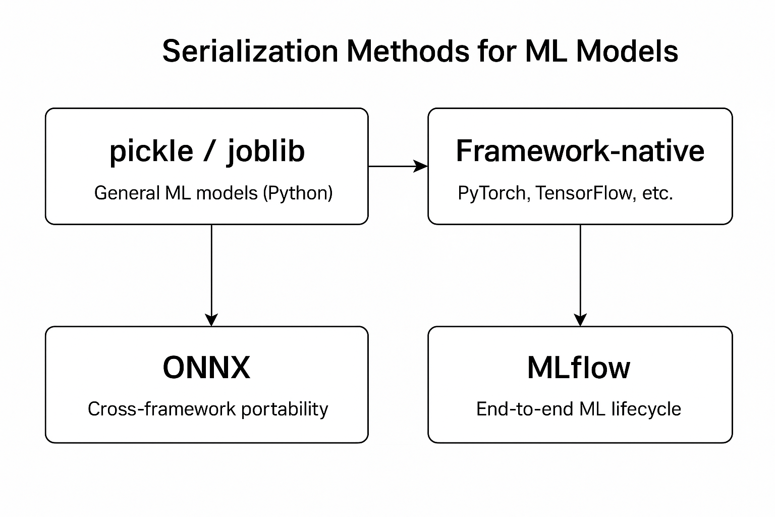
Serialization
The process of converting an in-memory object (e.g., a Python object) into a storable or transferable format (such as JSON, binary, or a file) so it can be saved or shared.
import json

data = {"name": "Ganesh", "course": "MLOps"}
# Serialization → Python dict → JSON string
serialized = json.dumps(data)

## Store the serialized data into JSON file if needed.
Deserialization
The process of converting the stored or transferred data (JSON, binary, file, etc.) back into an in-memory object that your program can use.
# Load it from JSON file
# Deserialization → JSON string → Python dict

deserialized = json.loads(serialized)
#serialization #deserialization #overfitting #underfitting
[Avg. reading time: 3 minutes]
Model vs Library vs Framework
python -m venv .demomodel
source .demomodel/bin/activate
pip install scikit-learn joblib
from sklearn.linear_model import LinearRegression
from sklearn.model_selection import train_test_split
from sklearn.metrics import mean_squared_error, r2_score
from joblib import dump, load
import numpy as np

# Fake dataset: study_hours -> exam_score
rng = np.random.default_rng(42)
hours = rng.uniform(0, 10, size=100).reshape(-1, 1)     # feature X
noise = rng.normal(0, 5, size=100)                      # noise
scores = 5 + 8*hours.ravel() + noise                    # target y

X_train, X_test, y_train, y_test =
    train_test_split(hours, scores, test_size=0.2, random_state=42)

model = LinearRegression()

# Train (fit)
model.fit(X_train, y_train)

# Evaluate
pred = model.predict(X_test)
print("MSE:", mean_squared_error(y_test, pred))
print("R2 :", r2_score(y_test, pred))
print("Learned slope and intercept:", model.coef_[0], model.intercept_)

# Save
dump(model, "linear_hours_to_score.joblib")

# Inference on new data
new_hours = np.array([[2.0], [5.0], [9.0]])
print("Predicted scores:", model.predict(new_hours))

# Predict after load

restored = load("linear_hours_to_score.joblib")
print("Loaded model predicts:", restored.predict(new_hours))
Fun Task
- Identify the Algorithj, Library, Model in this code
- What is MSE, R2_Score
- What is .joblib
- What is the number 42?
#model #library #framework #r2score #mse
[Avg. reading time: 2 minutes]
Explanation
-
Library: scikit-learn
-
Algorithm: Linear Regression (Mathematics)
-
Prebuilt Model: LinearRegression (part of scikit-learn library)
-
model.fit(): Custom built model for this data.
-
42 answer to the ultimate question of Life, the Universe, and Everything.
-
model.coef_[0] → the slope learned from data How much the target (exam score) increases for 1 extra unit of study hours model.intercept_ → the intercept The predicted target value when study hours = 0
Example:
Learned slope and intercept: 8.1 4.9
8.1 * hrs + 4.9
If a student studies 0 hours, predicted score ≈ 4.9 (baseline knowledge).
If a student studies 5 hours, predicted score ≈ 8.1 × 5 + 4.9 = 45.4.
[Avg. reading time: 3 minutes]
Statistical vs ML Models
Statistical Models
- Focus on inference -> understanding relationships between variables.
- Assume an underlying distribution (e.g., linear, normal).
- Typically work well with smaller datasets.
Goal: test hypotheses, estimate parameters.
Example: Linear regression to explain how income depends on education, experience, etc.
Machine Learning Models
- Focus on prediction -> finding patterns that generalize to unseen data.
- Fewer assumptions about data distribution.
- Can handle very large datasets and high-dimensional data.
Goal: optimize predictive performance.
Example: Random Forest predicting whether a customer will churn.
Key Similarities
Both use data to build models.
Both rely on training (fit) and evaluation (test).
Overlaps: linear regression is both a statistical model and an ML model, depending on context.
Book worth reading
The Manga Guide to Linear Algebra.
https://www.amazon.com/dp/1593274130
(Not an affiliate or referral)

On a lighter note
#statistics #ml #linearalgebra
[Avg. reading time: 3 minutes]
Types of ML Models
Supervised Learning
Data has input features (X) and target labels (y).
Model learns mapping: f(X) → y.
Examples:
- Regression -> Predicting house prices, demand forecast, server usage.
- Classification -> Spam vs Non-spam email or Customer churn.
Unsupervised Learning
Data has inputs only, no labels.
Goal: find hidden patterns or structure.
Examples:
- Clustering -> Customer segmentation.
- Association Rules -> Market basket analysis (“people who buy X also buy Y”).
- Dimensionality Reduction -> Principal Component Analysis (PCA) for visualization.
- Taking a high dimensional data and reducing it to fewer dimensions.
Reinforcement Learning (RL)
Agent interacts with environment -> learns by trial and error.
Used for decision-making & control.
Examples:
- Robotics & self-driving cars.
- Newer Video Games.
- OTT Content recommendations.
- Ads.
Semi-Supervised Learning
Mix of few labeled + many unlabeled data points.
Often used in NLP and computer vision.
Example: labeling 1,000 medical images, then using 100,000 unlabeled ones to improve model.
[Avg. reading time: 2 minutes]
ML Lifecycle
Collect Data (Data Engineers Role)
- Gather raw data from systems (databases, APIs, sensors, logs).
- Ensure sources are reliable and updated.
Clean & Prepare
- Handle missing values, outliers, and noise.
- Feature engineering: create new features, scale/encode as needed.
- Data splitting (train/validation/test).
Train Model
- Choose algorithm (supervised, unsupervised, reinforcement, etc.).
- Train on training set, tune hyperparameters.
Evaluate
- Use appropriate metrics:
- Classification → Accuracy, Precision, Recall, F1.
- Regression → RMSE, MAE, R².
- Cross-validation for robustness.
Deploy
- Make model accessible via API, batch jobs, or embedded in applications.
- Consider scaling (cloud, containers, edge devices).
Monitor & Improve
- Track data drift, concept drift, and model performance decay.
- Automate retraining pipelines (MLOps).
- Capture feedback loop to improve features and models.
#collect #clean #train #evaluate
[Avg. reading time: 6 minutes]
Data Preparation
~80% of the time in ML projects is spent on Data Preparation & Cleaning, and ~20% on Model Training.
The process of making raw data accurate, complete, and structured so it can be used for model training.
Wait data cleaning is not ML engineers job, it belongs to Data Engineer.
True but..
Data Engineers focus on collection and validation at scale:
- Ingest raw data from source systems (databases, APIs, IoT, logs).
- Build ETL/ELT pipelines (Bronze → Silver → Gold).
- Ensure data quality checks (avoid duplicates, schema validation, type checks, primary key uniqueness).
- Handle big data infrastructure: Spark, Databricks, Airflow, Kafka.
- Deliver curated data (often “Silver” or “Gold” layer) for downstream ML.
ML Engineers / Data Scientists take over once curated data is available:
- Apply ML-specific cleaning & prep:
- Impute missing values intelligently (mean/median/model-based).
- Encode categorical variables (one-hot, embeddings).
- Normalize/standardize numeric features.
- Text normalization, tokenization, embeddings.
- Create features meaningful to the ML model.
- Split data into train/validation/test sets.
flowchart LR
    DE[**Data Engineer**<br/><br/>- ETL/ELT Pipelines<br/>- Schema Validation<br/>• Deduplication<br/>- Type Checks]

    OVERLAP[**Common** <br/><br/>- Remove Duplicates<br/>- Ensure Consistency]

    MLE[**ML Engineer**<br/><br/>-Handle Missing Values<br/>- Feature Scaling<br/>- Imputation<br/>- Encoding & Embeddings<br/>- Train/Val/Test Split]

    DE --> OVERLAP
    MLE --> OVERLAP
For Example
Tabular Data
Data Engineer: ensures no duplicate customer IDs in database.
ML Engineer: fills missing “Age” values with median, scales “Income”.
Text Data
Data Engineer: stores raw customer reviews as UTF-8 encoded text.
ML Engineer: lowercases, removes stopwords, converts to embeddings.
Image Data
Data Engineer: validates images aren’t corrupted on ingest.
ML Engineer: resizes images, normalizes pixel values.
[Avg. reading time: 6 minutes]
Data Cleaning
Check for Target Leakage
What it is: Features that give away the answer (future info in training data).
Why it matters: Makes the model look perfect in training but useless in production.
Example:
When building a model having this column is not correct as in Production you will never have this during Prediction. This can be used when Testing your model prediction.
refund_issued_flag when predicting “Will this order be refunded?”.
Validate Labels
What it is: Make sure labels are correct, consistent, and usable.
Why it matters: Garbage labels = garbage predictions.
Example:
Churn column has values: yes, Y, 1, true.
Normalize to 1 = churn, 0 = not churn.
Handle Outliers Intentionally
What it is: Extreme values that distort training.
Why it matters: “Emp_Salary = 10,000,000” can throw off predictions.
Example
Cap at 99th percentile.
Flag as anomaly instead of training on it.
Enforce Feature Types
What it is: Make sure data types match their meaning.
Why it matters: Models can’t learn if types are wrong.
Example:
customer_id stored as integer → model may treat it as numeric.
Why is that problem, customer_id = 20 will have more weightage than customer_id = 1
Convert to string (categorical).
Standardize Categories
What it is: Inconsistent labels in categorical columns.
Why it matters: Model may treat the same thing as different classes.
Example:
Country: USA, U.S.A., United States.
Map all to United States.
Normalize Text for ML
What it is: Clean and standardize text features.
Why it matters: Prevents the model from treating “Hello” and “hello!” as different.
Example:
Lowercasing, removing punctuation, stripping whitespace.
Keep a copy of raw text for audit.
Protect Data Splits
What it is: Make sure related rows don’t leak between train/test.
Why it matters: Prevents unfair accuracy boost.
Example:
Same student appears in both train and test sets.
Fix: Group by student_id when splitting.
#datacleaning #mlcleaning #normalize_data
[Avg. reading time: 11 minutes]
Data Imputation
Data Imputation is the process of filling in missing values in a dataset with estimated or predicted values.
Data imputation aims to enhance the quality and completeness of the dataset, ultimately improving the performance and reliability of the ML model.
Problems with Missing Data
- Reduced Model
- Biased Inferences
- Imbalanced Representations
- Increased complexity in Model handling
Data Domain knowledge is important before choosing the right method.
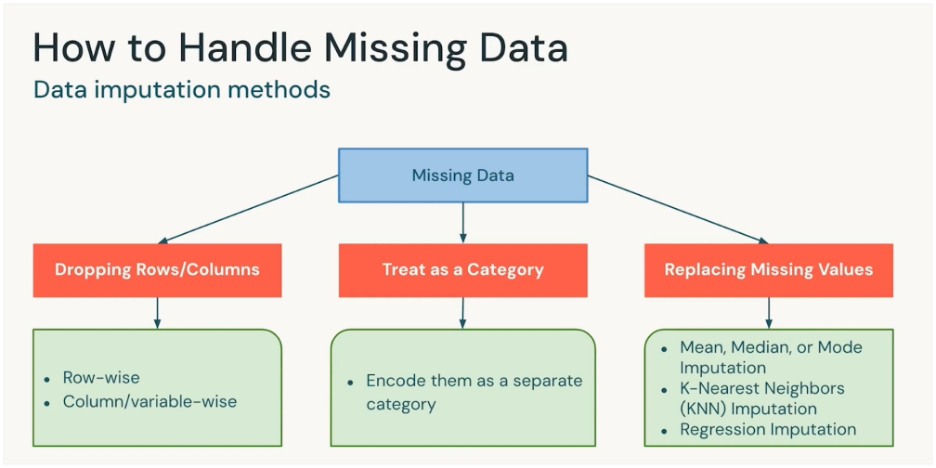
Dropping Rows/Columns
Remove the rows or columns that contain missing values.
- If the percentage of missing data is very small.
- If the column isn’t important for the model.
Example: Drop the few rows out of Million where “Age” is missing.
Treat as a Category
Encode “missing” or “NA” or “Unknown” as its own category.
- For categorical variables (like Country, Gender, Payment Method).
When “missing” itself carries meaning (e.g., customer didn’t provide income → may be sensitive).
Example: Add a category Unknown to “Marital Status” column.
Data with Missing Values
| ID | Country |
|---|---|
| 1 | USA |
| 2 | Canada |
| 3 | Null |
| 4 | India |
| 5 | NA (missing) |
After treating as a Category
| ID | Country |
|---|---|
| 1 | USA |
| 2 | Canada |
| 3 | Missing |
| 4 | India |
| 5 | Missing |
The model will see “Missing” as just another value like “USA” or “India.”
Replacing Missing Values (Imputation)
Fill missing values with a reasonable estimate.
Methods:
- Mean/Median/Mode: Quick fixes for numeric/categorical data.
- KNN Imputation: Fill value based on “closest” similar records.
- Regression Imputation: Predict the missing value using other features.
Example: Replace missing “Salary” with median salary of the group.
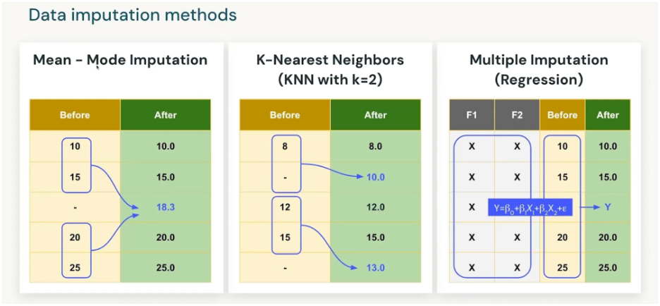
Using regression models repeatedly (with randomness) to fill missing data, producing several plausible datasets, and then combining them for analysis.
| Age | Education | Income |
|---|---|---|
| 30 | Masters | ? |
| 40 | PhD | 120K |
| 35 | Bachelors | 80K |
- Step 1: Fit regression: Income ~ Age + Education.
- Step 2: Predict missing Income for Age=30, Edu=Masters.
- Step 3: Add random noise → 95K in dataset1, 92K in dataset2, 98K in dataset3.
- Step 4: Analyze all 3 datasets, combine results.
Downside: Delay in process and computing time. More missing values more coputation time.
- Drop : if it’s tiny and negligible.
- Category : if it’s categorical.
- Replace : if it’s numeric and important.
- KNN/Regression : if you want smarter imputations and can afford compute.
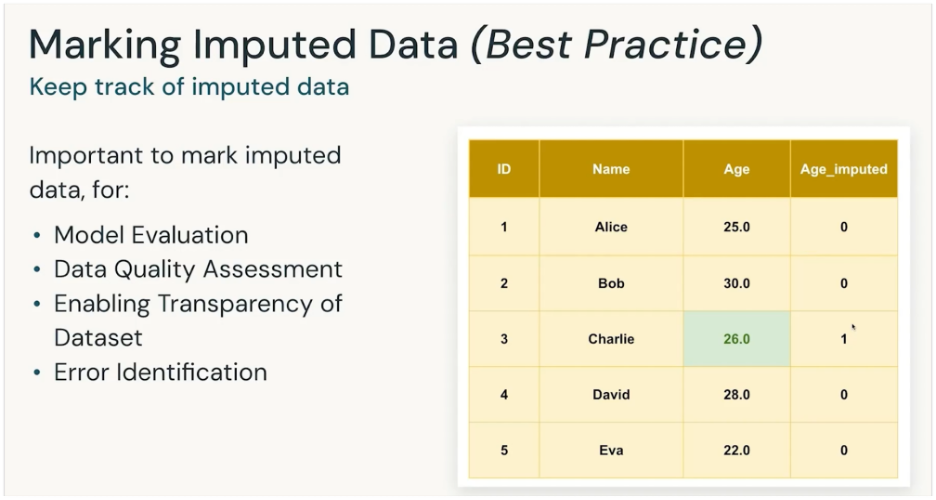
It is important to mark the imputated data
To know which data is from source and which is calculated. So its handled with pinch of salt.
| Method | When to Use | Pros | Cons |
|---|---|---|---|
| Drop Rows/Columns | When % of missing data is very small (e.g., <5%) or the feature is unimportant | - Simple and fast - No assumptions needed | - Lose data (rows) - Risk of losing valuable features (columns) |
| Treat as a Category | For categorical variables where “missing” may carry meaning | - Preserves all rows - Captures the “missingness” as useful info | - Only works for categorical data - Can create an artificial category if missing isn’t meaningful |
| Replace with Mean/Median/Mode | For numeric data (mean/median) or categorical (mode) | - Easy to implement - Keeps dataset size intact | - Distorts distribution - Ignores correlations between features |
| KNN Imputation | When dataset is not too large and similar neighbors make sense | - Considers relationships between features - More accurate than simple averages | - Computationally expensive - Sensitive to scaling and choice of K |
| Regression Imputation | When missing values can be predicted from other variables | - Uses feature relationships - Can be very accurate | - Risk of “overfitting” imputations - Adds complexity |
#dataimputation #knn #encode #dropdata
[Avg. reading time: 13 minutes]
Data Encoding
Data Encoding is the process of converting categorical data (like colors, countries, product types) into a numeric format that ML models can understand.
Unlike numerical data, categorical data is not directly usable because models operate on numbers, not labels.
Encoding ensures categorical values are represented in a way that preserves meaning and avoids misleading the model.
Typically rule-based.
Example: Products
| ID | Product |
|---|---|
| 1 | Laptop |
| 2 | Phone |
| 3 | Tablet |
| 4 | Phone |
Label Encoding
Assigns each category a unique integer.
| ID | Product (Encoded) |
|---|---|
| 1 | 0 |
| 2 | 1 |
| 3 | 2 |
| 4 | 1 |
Pros:
- Very simple, minimal storage.
- Works well for tree-based models.
Cons:
- Implies an order between categories (Laptop < Phone < Tablet).
- Misleads linear models.
One-Hot Encoding
Creates a binary column for each category.
| ID | Laptop | Phone | Tablet |
|---|---|---|---|
| 1 | 1 | 0 | 0 |
| 2 | 0 | 1 | 0 |
| 3 | 0 | 0 | 1 |
| 4 | 0 | 1 | 0 |
Pros:
- No ordinal assumption.
- Easy to interpret.
Cons:
- High dimensionality for many products (e.g., thousands of SKUs).
- Sparse data, more memory needed.
Ordinal Encoding
Encodes categories when they have a natural order.
Works for things like product size or version level.
Example (Product Tier):
| ID | Product Tier |
|---|---|
| 1 | Basic |
| 2 | Standard |
| 3 | Premium |
| 4 | Standard |
After Ordinal Encoding:
| ID | Product Tier (Encoded) |
|---|---|
| 1 | 1 |
| 2 | 2 |
| 3 | 3 |
| 4 | 2 |
Pros:
- Preserves rank/order.
- Efficient storage.
Cons:
- Only valid if order is real (Basic < Standard < Premium).
- Wrong if categories are unordered (Laptop vs Phone).
Target Encoding (Mean Encoding)
Replaces each category with the mean of the target variable.
Target - “Purchased” Yes=1, No=0
| ID | Product | Purchased |
|---|---|---|
| 1 | Laptop | 1 |
| 2 | Phone | 0 |
| 3 | Tablet | 1 |
| 4 | Phone | 1 |
| ID | Product (Encoded) | Purchased |
|---|---|---|
| 1 | 1.0 | 1 |
| 2 | 0.5 | 0 |
| 3 | 1.0 | 1 |
| 4 | 0.5 | 1 |
Compute mean purchase rate:
Laptop = 1.0 Phone = 0.5 Tablet = 1.0
Pros:
- Great for high-cardinality features (e.g., hundreds of product SKUs).
- Often improves accuracy.
- Keeps dataset compact (just 1 numeric column).
- Often boosts performance in models like Logistic Regression or Gradient Boosted Trees.
Cons:
- Risk of data leakage if target encoding is done on the whole dataset.
- Must use cross-validation to avoid leakage.
- Compute intensive.
| Encoding Type | Best For | Avoid When |
|---|---|---|
| Label Encoding | Tree-based models, low-cardinality products | Linear models, unordered categories |
| One-Hot Encoding | General ML, few product categories | Very high-cardinality features |
| Ordinal Encoding | Ordered categories (tiers, sizes, versions) | Unordered categories (Phone vs Laptop) |
| Target Encoding | High-cardinality products, with proper CV | Without CV (leakage risk) |
Multiple Categorical Columns
| ID | Product | Product Tier | Category | Purchased |
|---|---|---|---|---|
| 1 | Laptop | Premium | PC | 1 |
| 2 | Phone | Basic | Mobile | 0 |
| 3 | Tablet | Standard | Electronics | 1 |
| 4 | Phone | Premium | Mobile | 1 |
- Product: Laptop, Phone, Tablet
- Product Tier: Basic < Standard < Premium (ordered)
- Category: Electronics, Accessories, Clothing (unordered)
Label Encoding (all columns)
Replace each category with an integer.
| ID | Product | Product Tier | Category |
|---|---|---|---|
| 1 | 0 | 2 | 0 |
| 2 | 1 | 0 | 1 |
| 3 | 2 | 1 | 2 |
| 4 | 1 | 2 | 1 |
Artificial order created (e.g., PC=0, Mobile=1, Electronics=2).
One-Hot Encoding (all columns)
| ID | Laptop | Phone | Tablet | Tier_Basic | Tier_Standard | Tier_Premium | Cat_PC | Cat_Mobile | Cat_Electronics |
|---|---|---|---|---|---|---|---|---|---|
| 1 | 1 | 0 | 0 | 0 | 0 | 1 | 1 | 0 | 0 |
| 2 | 0 | 1 | 0 | 1 | 0 | 0 | 0 | 1 | 0 |
| 3 | 0 | 0 | 1 | 0 | 1 | 0 | 0 | 0 | 1 |
| 4 | 0 | 1 | 0 | 0 | 0 | 1 | 0 | 1 | 0 |
Very interpretable, but column explosion if you have 50+ products or 100+ categories.
Mixed Encoding (best practice)
- Product → One-Hot (few categories).
- Product Tier → Ordinal (Basic=1, Standard=2, Premium=3).
- Category → One-Hot (PC, Mobile, Electronics).
| ID | Laptop | Phone | Tablet | Tier (Ordinal) | Cat_PC | Cat_Mobile | Cat_Electronics |
|---|---|---|---|---|---|---|---|
| 1 | 1 | 0 | 0 | 3 | 1 | 0 | 0 |
| 2 | 0 | 1 | 0 | 1 | 0 | 1 | 0 |
| 3 | 0 | 0 | 1 | 2 | 0 | 0 | 1 |
| 4 | 0 | 1 | 0 | 3 | 0 | 1 | 0 |
#onehot_encoding #target_encoding #label_encoding
[Avg. reading time: 6 minutes]
Feature Engineering
The process of transforming raw data into more informative inputs (features) for ML models.
Goes beyond encoding: you can create new features/metrics (like derived columns in the DB world) that pure encoding does not offer.
The goal of FE is to improve model accuracy, interpretability, and generalization.
Example (Laptop Sales):
Purchase Date = 2025-09-02
Derived Features:
- Month = 09
- DayOfWeek = Tuesday
- IsHolidaySeason = No
- IsWeekend = No
- IsLeapYear= No
- Quarter = Q3
Encoding (One-Hot, Label, Target) = only turns categories into numbers.
But real-world data often hides useful patterns in dates, interactions, domain knowledge, or semantics.
| ID | Product | Purchase Date | Price | PurchasedAgain |
|---|---|---|---|---|
| 1 | Laptop | 2023-12-01 | 1200 | 1 |
| 2 | Laptop | 2024-07-15 | 1100 | 0 |
| 3 | Phone | 2024-05-20 | 800 | 1 |
| 4 | Tablet | 2024-08-05 | 600 | 1 |
- Encoding only handles Product → One-Hot or Target.
Feature Engineering adds new insights:
- From Purchase Date: extract Month, DayOfWeek, IsHolidaySeason.
- From Price: create Discounted? (if < avg product price).
- Combine features: Price / AvgCategoryPrice.
Basic Feature Engineering
Improve signals/patterns without domain-specific knowledge.
Scaling/Normalization: Price → (Price – mean) / std
Date/Time Features: Purchase Date → Month=12, DayOfWeek=Friday
Polynomial/Interaction: Price × Tier
Pros:
- Easy to implement.
- Immediately boosts many models (especially linear/Neural Networks).
Cons:
- Risk of adding noise if done blindly.
- Limited unless combined with domain insights.
Domain-Specific Feature Engineering
Apply business/field knowledge.
Examples:
Finance: Debt-to-Income Ratio, Credit Utilization %
Healthcare: BMI = Weight / Height², risk score categories
IoT: Rolling averages, peak detection in sensor data.
Pros:
- Captures real-world meaning → big performance gains.
- Makes models explainable to stakeholders.
Cons:
- Requires domain expertise.
- Not always transferable between datasets.
#feature_engineering #domain_specific
[Avg. reading time: 10 minutes]
Vectors
A vector is just an ordered list of numbers that represents a data point so models can do math on it.
Think “row -> numbers” for tabular data, or “text/image -> numbers” after a transformation.
Example:
Price = 1200, Weight = 2kg, Warranty = 24 months → Vector = [1200, 2, 24]
Types of Vectors
Tabular Feature Vector
Concatenate numeric columns (and encoded categoricals) into a single vector.
ML engineer/data scientist during data prep/FE (training) and the same code at inference.
Example: [Price, Weight, Warranty] → [1200, 2, 24].
Sparse Vectors
High-dimensional vectors with many zeros (e.g., One-Hot, Bag-of-Words, TF-IDF).
Encoding/featurization function in your pipeline.
Example
Products = {Laptop, Phone, Pen}
Laptop → [1, 0, 0]
Phone → [0, 1, 0]
Pen → [0, 0, 1]
Dense Vectors (compact, mostly non-zeros)
Lower-dimensional, compact numeric representation
Created by algorithms (scalers/PCA) or models (embeddings) in your pipeline.
Lower-dimensional, compact, mostly non-zeros → dense.
Example: Not actual values
Laptop → [0.65, -0.12, 0.48]
Phone → [0.60, -0.15, 0.52]
Pen → [0.10, 0.85, -0.40]
Laptop and Phone vectors are close together.
Model-Derived Feature Vectors
Dense vectors specifically generated by models like CNN/Transformer as a vector. Mainly used with Computer Vision. Image classification, object detection, face recognition, voice processing.
Models generate them during feature extraction (training & inference).
Example: BERT sentence vector, ResNet image features.
| Vector Type | Who designs it? | Who computes it? | When it’s computed | Example |
|---|---|---|---|---|
| Tabular feature vector | ML Eng/DS (choose columns) | Pipeline code | Train & Inference | [Price, Weight, Warranty] |
| Sparse (One-Hot/TF-IDF) | ML Eng/DS (choose encoder) | Encoder in pipeline | Train (fit) & Inference (transform) | One-Hot Product |
| Dense (scaled/PCA) | ML Eng/DS (choose scaler/PCA) | Scaler/PCA in pipeline | Train (fit) & Inference (transform) | StandardScaled price, PCA(100) |
| Model features / Embeddings | ML Eng/DS (choose model) | Model (pretrained or trained) | Train & Inference | BERT/ResNet/categorical embedding |
MLOps ensures the same steps run at inference to avoid train/serve skew.
Example of Dense Vector
python -m venv .densevector
source .densevector/bin/activate
pip install sentence-transformers
from sentence_transformers import SentenceTransformer

# Load a pre-trained model (MiniLM is small & fast)
model = SentenceTransformer('all-MiniLM-L6-v2')

text = "Laptop"

# Convert text into dense vector
vector = model.encode(text)

print("Dense Vector Shape:", text, vector.shape)
print("Dense Vector (first 10 values):", vector[:10])
from sentence_transformers import SentenceTransformer
from sklearn.metrics.pairwise import cosine_similarity
import numpy as np

# Load model
model = SentenceTransformer('all-MiniLM-L6-v2')

# Words
texts = ["Laptop", "Computer", "Pencil"]

# Encode all
vectors = model.encode(texts)

# Convert to numpy array
vectors = np.array(vectors)

# Cosine similarity matrix
sim_matrix = cosine_similarity(vectors)

# Display similarity scores
for i in range(len(texts)):
    for j in range(i+1, len(texts)):
        print(f"Similarity({texts[i]} vs {texts[j]}): {sim_matrix[i][j]:.4f}")
#vectors #densevector #sparsevector #tabularvector
[Avg. reading time: 8 minutes]
Embeddings
Embeddings transform high-dimensional categorical or textual data into a compact, dense vector space.
Similar items are placed closer together in vector space -> models can understand similarity.
- These representations capture relationships and context among different entities.
- Used in Recommendation Systems, NLP, Image Search and more.
- Can be learning from data using neural networks or retrieved from pretrained models (eg: Word2Vec, FastText)
Use Cases
- Search & Retrieval: Semantic search, image search.
- NLP: Word/sentence embeddings for sentiment, chatbots, translation.
- Computer Vision: Image embeddings for similarity or classification.
Advantages over traditional encoding:
- Handle high-cardinality categorical features (e.g., millions of products).
- Capture context and semantics (“Laptop” is closer to “Computer” than “Pencil”).
- Lower-dimensional → more efficient than One-Hot or TF-IDF.
Types of Embeddings
Word Embeddings (Text)
Represent words as vectors so that semantically similar words are close together.
Examples: Word2Vec, GloVe, FastText.
“king” – “man” + “woman” = “queen”
Used in: sentiment analysis, translation, chatbots.
Sentence / Document Embeddings (Text)
Represent longer text (sentences, paragraphs, docs) in vector form.
Capture context and meaning beyond individual words.
Examples: BERT, Sentence-BERT, Universal Sentence Encoder.
“The laptop is fast” and “This computer is quick” → close vectors.
Image Embeddings (Computer Vision)
Represent images as vectors extracted from CNNs or Vision Transformers.
Capture visual similarity (shapes, colors, objects).
Examples: ResNet, CLIP (image+text).
A cheetah photo and a leopard photo → embeddings close together (both cat family).
Used in: image search, face recognition, object detection.
Audio / Speech Embeddings
Convert audio waveforms into dense vectors capturing phonetics and semantics.
Examples: wav2vec, HuBERT.
Voice saying “Laptop” → embedding close to text embedding of “Laptop”.
Used in: speech recognition, speaker identification.
Graph Embeddings
Represent nodes/edges in a graph (social networks, knowledge graphs).
Capture relationships and network structure.
Examples: Node2Vec, DeepWalk, Graph Neural Networks (GNNs).
In a product graph, Laptop node embedding will be close to Mouse if often co-purchased.
| Type | Example Algorithms | Data Type | Use Cases |
|---|---|---|---|
| Word | Word2Vec, GloVe | Text (words) | NLP basics |
| Sentence/Doc | BERT, SBERT | Text (longer) | Semantic search, QA |
| Categorical | Embedding layers | Tabular (IDs) | Recommenders, fraud detection |
| Image | ResNet, CLIP | Vision | Image search, recognition |
| Audio | wav2vec, HuBERT | Audio | Speech-to-text, voice auth |
| Graph | Node2Vec, GNNs | Graphs | Social networks, KG search |
#embeddings [#<abbr title="Bidirectional Encoder Representations from Transformers">BERT</abbr>](../tags.md#BERT "Tag: BERT") #Word2Vec #NLP
[Avg. reading time: 7 minutes]
Life Before MLOps
Challenges Faced by ML Teams.
Moving Models from Dev → Staging → Prod
Models were often shared as .pkl or joblib files, passed around manually.
Problem: Dependency mismatches (Python, sklearn version), fragile handoffs.
Stopgap: Packaging models with Docker images, but still manual and inconsistent.
Champion vs Challenger Deployment
Teams struggled to test a new (challenger) model against the current (champion).
Problem: No controlled A/B testing or shadow deployments → risky rollouts.
Stopgap: Manual canary releases or running offline comparisons.
Model Versioning Confusion
Models saved as model_final.pkl, model_final_v2.pkl, final_final.pkl.
Problem: Nobody knew which version was truly in production.
Stopgap: Git or S3 versioning for files, but no link to experiments/data.
Inference on Wrong Model Version
Even if multiple versions existed, production systems sometimes pointed to the wrong one.
Problem: Silent failures, misaligned experiments vs prod results.
Stopgap: Hardcoding file paths or timestamps — brittle and error-prone.
Train vs Serve Skew (Data-Model Mismatch)
Preprocessing done in notebooks was re-written differently in prod code.
Problem: Same model behaves differently in production.
Stopgap: Copy-paste code snippets, but no guarantee of sync.
Experiment Tracking Chaos
Results scattered across notebooks, Slack messages, spreadsheets.
Problem: Couldn’t reproduce “that good accuracy we saw last week.”
Stopgap: Manually logging metrics in Excel or text files.
Reproducibility Issues
Same code/data gave different results on different machines.
Problem: No control of data versions, package dependencies, or random seeds.
Stopgap: Virtualenvs, requirements.txt — helped a bit but not full reproducibility.
Lack of Monitoring in Production
Once deployed, no one knew if the model degraded over time.
Problem: Models silently failed due to data drift or concept drift.
Stopgap: Occasional manual performance checks, but no automation.
Scaling & Performance Gaps
Models trained in notebooks failed under production loads.
Problem: Couldn’t handle large-scale data or real-time inference.
Stopgap: Batch scoring jobs on cron — but too slow for real-time use cases.
Collaboration Breakdowns
Data Scientists, Engineers, Ops worked in silos.
Problem: Miscommunication -> wrong datasets, broken pipelines, delays.
Stopgap: Jira tickets and handovers — but still slow and error-prone.
Governance & Compliance Gaps
No audit trail of which model made which prediction.
Problem: Risky for regulated domains (finance, healthcare).
Stopgap: Manual logging of predictions — incomplete and unreliable.
#mlops #development #production
[Avg. reading time: 13 minutes]
Quiz
Note: This is a practice quiz and will not be graded. The purpose is to help you check your understanding of the concepts we covered.
[Avg. reading time: 0 minutes]
Developer Tools
[Avg. reading time: 5 minutes]
Introduction
Before diving into Data or ML frameworks, it's important to have a clean and reproducible development setup. A good environment makes you:
- Faster: less time fighting dependencies.
- Consistent: same results across laptops, servers, and teammates.
- Confident: tools catch errors before they become bugs.
A consistent developer experience saves hours of debugging. You spend more time solving problems, less time fixing environments.
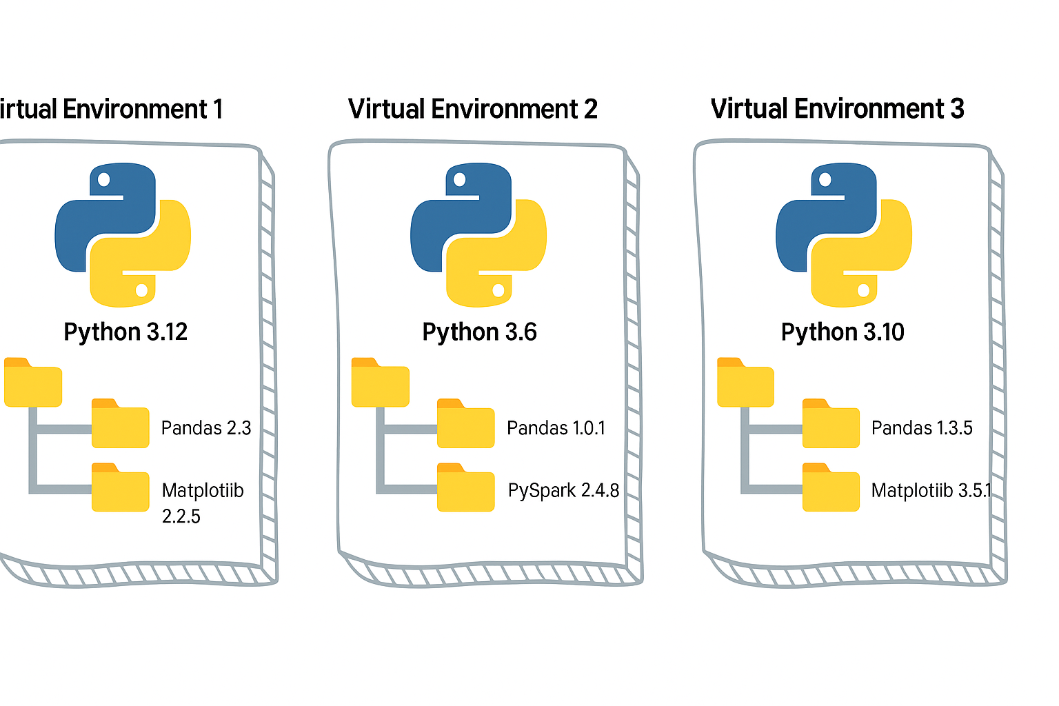
Python Virtual Environment
- A virtual environment is like a sandbox for Python.
- It isolates your project’s dependencies from the global Python installation.
- Easy to manage different versions of library.
- Must depend on requirements.txt, it has to be managed manually.
Without it, installing one package for one project may break another project.
Open the CMD prompt (Windows)
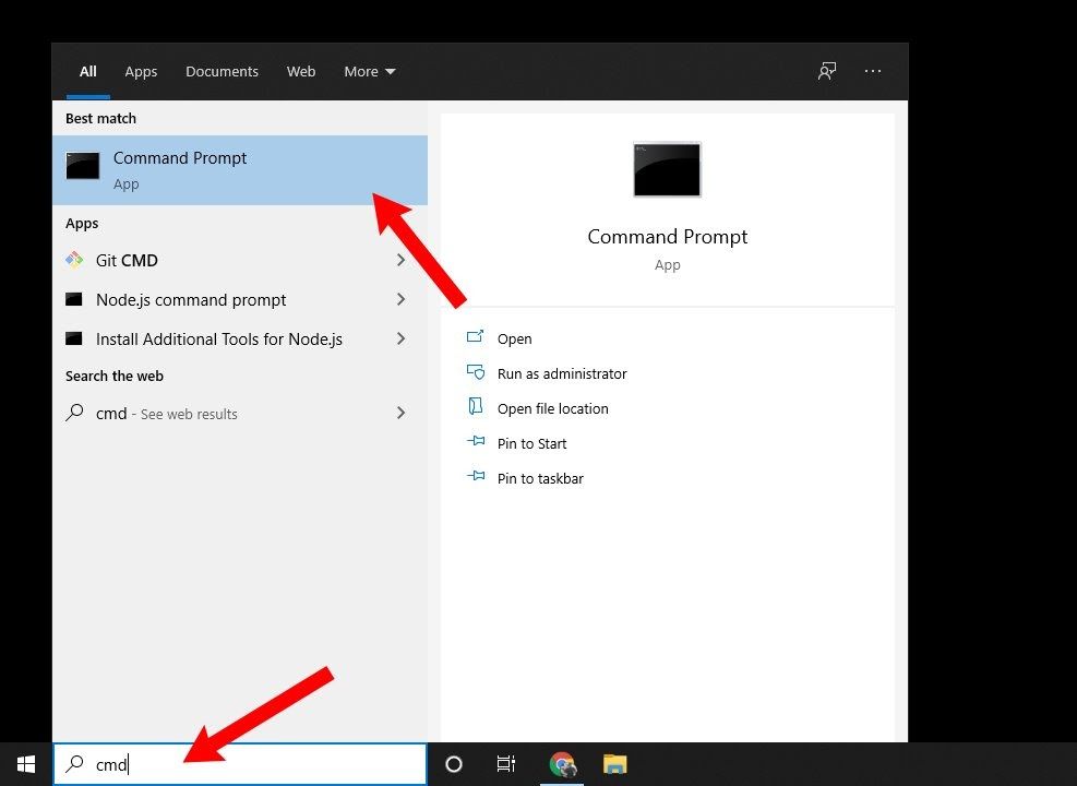
Open the Terminal (Mac)

# Step 0: Create a project folder under your Home folder.

mkdir project

cd project


# Step 1: Create a virtual environment
python -m venv myenv

# Step 2: Activate it
# On Mac/Linux:
source myenv/bin/activate

# On Windows:
myenv\Scripts\activate.bat

# Step 3: Install packages (they go inside `myenv`, not global)
pip install faker

# Step 4: Open Python
python

# Step 5: Verify

import sys

sys.prefix

sys.base_prefix

# Step 6: Run this sample

from faker import Faker
fake = Faker()
fake.name()

# Step 6: Close Python (Control + Z)

# Step 7: Deactivate the venv when done

deactivate
As a next step, you can either use Poetry or UV as your package manager.
#venv #python #uv #poetry developer_tools
[Avg. reading time: 3 minutes]
UV
Dependency & Environment Manager
- Written in Rust.
- Syntax is lightweight.
- Automatic Virtual environment creation.
Create a new project:
# Initialize a new uv project
uv init uv_helloworld
Sample layout of the directory structure
.
├── main.py
├── pyproject.toml
├── README.md
└── uv.lock
# Change directory
cd uv_helloworld

# # Create a virtual environment myproject
# uv venv myproject

# or create a UV project with specific version of Python

# uv venv myproject --python 3.11

# # Activate the Virtual environment

# source myproject/bin/activate

# # Verify the Virtual Python version

# which python3

# add library (best practice)
uv add faker

# verify the list of libraries under virtual env
uv tree

# To find the list of libraries inside Virtual env

uv pip list
edit the main.py
from faker import Faker
fake = Faker()
print(fake.name())
uv run main.py
Read More on the differences between UV and Poetry
[Avg. reading time: 12 minutes]
Python Developer Tools
PEP
PEP, or Python Enhancement Proposal, is the official style guide for Python code. It provides conventions and recommendations for writing readable, consistent, and maintainable Python code.
- PEP 8 : Style guide for Python code (most famous).
- PEP 20 : "The Zen of Python" (guiding principles).
- PEP 484 : Type hints (basis for MyPy).
- PEP 517/518 : Build system interfaces (basis for pyproject.toml, used by Poetry/UV).
- PEP 572 : Assignment expressions (the := walrus operator).
- PEP 695 : Type parameter syntax for generics (Python 3.12).
Key Aspects of PEP 8 (Popular ones)
Indentation
- Use 4 spaces per indentation level
- Continuation lines should align with opening delimiter or be indented by 4 spaces.
Line Length
- Limit lines to a maximum of 79 characters.
- For docstrings and comments, limit lines to 72 characters.
Blank Lines
- Use 2 blank lines before top-level functions and class definitions.
- Use 1 blank line between methods inside a class.
Imports
- Imports should be on separate lines.
- Group imports into three sections: standard library, third-party libraries, and local application imports.
- Use absolute imports whenever possible.
# Correct
import os
import sys

# Wrong
import sys, os
Naming Conventions
- Use
snake_casefor function and variable names. - Use
CamelCasefor class names. - Use
UPPER_SNAKE_CASEfor constants. - Avoid single-character variable names except for counters or indices.
Whitespace
- Don’t pad inside parentheses/brackets/braces.
- Use one space around operators and after commas, but not before commas.
- No extra spaces when aligning assignments.
Comments
- Write comments that are clear, concise, and helpful.
- Use complete sentences and capitalize the first word.
- Use # for inline comments, but avoid them where the code is self-explanatory.
Docstrings
- Use triple quotes (""") for multiline docstrings.
- Describe the purpose, arguments, and return values of functions and methods.
Code Layout
- Keep function definitions and calls readable.
- Avoid writing too many nested blocks.
Consistency
- Consistency within a project outweighs strict adherence.
- If you must diverge, be internally consistent.
Linting
Linting is the process of automatically checking your Python code for:
-
Syntax errors
-
Stylistic issues (PEP 8 violations)
-
Potential bugs or bad practices
-
Keeps your code consistent and readable.
-
Helps catch errors early before runtime.
-
Encourages team-wide coding standards.
# Incorrect
import sys, os

# Correct
import os
import sys
# Bad spacing
x= 5+3

# Good spacing
x = 5 + 3
Ruff : Linter and Code Formatter
Ruff is a fast, modern tool written in Rust that helps keep your Python code:
- Consistent (follows PEP 8)
- Clean (removes unused imports, fixes spacing, etc.)
- Correct (catches potential errors)
Install
poetry add ruff
uv add ruff
Verify
ruff --version
ruff --help
example.py
import os, sys

def greet(name):
  print(f"Hello, {name}")

def message(name): print(f"Hi, {name}")

def calc_sum(a, b): return a+b

greet('World')
greet('Ruff')
message('Ruff')
poetry run ruff check example.py
poetry run ruff check example.py --fix

poetry run ruff format example.py --check
poetry run ruff format example.py
OR
uv run ruff check example.py
uv run ruff check example.py --fix
uv run ruff format example.py --check
uv run ruff check example.py
MyPy : Type Checking Tool
mypy is a static type checker for Python. It checks your code against the type hints you provide, ensuring that the types are consistent throughout the codebase.
It primarily focuses on type correctness—verifying that variables, function arguments, return types, and expressions match the expected types.
Install
    poetry add mypy

    or

    uv add mypy

    or

    pip install mypy
sample.py
x = 1
x = 1.0
x = True
x = "test"
x = b"test"

print(x)

def add(a: int, b: int) -> int:
    return a + b

print(add(100, 123))

print(add("hello", "world"))
uv run mypy sample.py

or

poetry run mypy sample.py

or

mypy sample.py
[Avg. reading time: 8 minutes]
Error Handling
Python uses try/except blocks for error handling.
The basic structure is:
try:
    # Code that may raise an exception
except ExceptionType:
    # Code to handle the exception
finally:
    # Code executes all the time
Uses
Improved User Experience: Instead of the program crashing, you can provide a user-friendly error message.
Debugging: Capturing exceptions can help you log errors and understand what went wrong.
Program Continuity: Allows the program to continue running or perform cleanup operations before terminating.
Guaranteed Cleanup: Ensures that certain operations, like closing files or releasing resources, are always performed.
Some key points
-
You can catch specific exception types or use a bare except to catch any exception.
-
Multiple except blocks can be used to handle different exceptions.
-
An else clause can be added to run if no exception occurs.
-
A finally clause will always execute, whether an exception occurred or not.
Without Try/Except
x = 10 / 0
Basic Try/Except
try:
    x = 10 / 0
except ZeroDivisionError:
    print("Error: Division by zero!")
Generic Exception
try:
    file = open("nonexistent_file.txt", "r")
except:
    print("An error occurred!")
Find the exact error
try:
    file = open("nonexistent_file.txt", "r")
except Exception as e:
    print(str(e))
Raise - Else and Finally
try:
    x = -10
    if x <= 0:
        raise ValueError("Number must be positive")
except ValueError as ve:
    print(f"Error: {ve}")
else:
    print(f"You entered: {x}")
finally:
    print("This will always execute")
try:
    x = 10
    if x <= 0:
        raise ValueError("Number must be positive")
except ValueError as ve:
    print(f"Error: {ve}")
else:
    print(f"You entered: {x}")
finally:
    print("This will always execute")
Nested Functions
def divide(a, b):
    try:
        result = a / b
        return result
    except ZeroDivisionError:
        print("Error in divide(): Cannot divide by zero!")
        raise  # Re-raise the exception

def calculate_and_print(x, y):
    try:
        result = divide(x, y)
        print(f"The result of {x} divided by {y} is: {result}")
    except ZeroDivisionError as e:
        print(str(e))
    except TypeError as e:
        print(str(e))

# Test the nested error handling
print("Example 1: Valid division")
calculate_and_print(10, 2)

print("\nExample 2: Division by zero")
calculate_and_print(10, 0)

print("\nExample 3: Invalid type")
calculate_and_print("10", 2)
[Avg. reading time: 4 minutes]
UnitTest
A unit test verifies the correctness of a small, isolated "unit" of code—typically a single function or method—independent of the rest of the program.
Key Benefits of Unit Testing
Isolates functionality – Tests focus on one unit at a time, making it easier to pinpoint where a bug originates.
Enables early detection – Issues are caught during development, reducing costly fixes later in production.
Prevents regressions – Running existing tests after changes ensures new bugs aren’t introduced.
Supports safe refactoring – With a strong test suite, developers can confidently update or restructure code.
Improves quality – High coverage enforces standards, highlights edge cases, and strengthens overall reliability.
Unit Testing in Python
Every language provides its own frameworks for unit testing. In Python, popular choices include:
unittest – The built-in testing framework in the standard library.
pytest – Widely used, simple syntax, rich plugin ecosystem.
doctest – Tests embedded directly in docstrings.
testify – An alternative framework inspired by unittest, with added features.
pytest is the popular testing tool for data/ML code. It’s faster to write, far more expressive for data-heavy tests, and has a rich plugin ecosystem that plays nicely with Spark, Pandas, MLflow, and CI.
git clone https://github.com/gchandra10/pytest-demo.git
uv run pytest -v
[Avg. reading time: 11 minutes]
DUCK DB
DuckDB is a single file built with no dependencies.
All the great features can be read here https://duckdb.org/
Automatic Parallelism: DuckDB has improved its automatic parallelism capabilities, meaning it can more effectively utilize multiple CPU cores without requiring manual tuning. This results in faster query execution for large datasets.
Parquet File Improvements: DuckDB has improved its handling of Parquet files, both in terms of reading speed and support for more complex data types and compression codecs. This makes DuckDB an even better choice for working with large datasets stored in Parquet format.
Query Caching: Improves the performance of repeated queries by caching the results of previous executions. This can be a game-changer for analytics workloads with similar queries being run multiple times.
How to use DuckDB?
Download the CLI Client
-
Linux).
-
For other programming languages, visit https://duckdb.org/docs/installation/
-
Unzip the file.
-
Open Command / Terminal and run the Executable.
DuckDB in Data Engineering
Download orders.parquet from
https://github.com/duckdb/duckdb-data/releases/download/v1.0/orders.parquet
More files are available here
https://github.com/cwida/duckdb-data/releases/
Open Command Prompt or Terminal
./duckdb
# Create / Open a database

.open ordersdb
Duckdb allows you to read the contents of orders.parquet as is without needing a table. Double quotes around the file name orders.parquet is essential.
describe table "orders.parquet"
Not only this, but it also allows you to query the file as-is. (This feature is similar to one data bricks supports)
select * from "orders.parquet" limit 3;
DuckDB supports CTAS syntax and helps to create tables from the actual file.
show tables;

create table orders  as select * from "orders.parquet";

select count(*) from orders;
DuckDB supports parallel query processing, and queries run fast.
This table has 1.5 million rows, and aggregation happens in less than a second.
select now(); select o_orderpriority,count(*) cnt from orders group by o_orderpriority; select now();
DuckDB also helps to convert parquet files to CSV in a snap. It also supports converting CSV to Parquet.
COPY "orders.parquet" to 'orders.csv' (FORMAT "CSV", HEADER 1);Select * from "orders.csv" limit 3;
It also supports exporting existing Tables to Parquet files.
COPY "orders" to 'neworder.parquet' (FORMAT "PARQUET");
DuckDB supports Programming languages such as Python, R, JAVA, node.js, C/C++.
DuckDB ably supports Higher-level SQL programming such as Macros, Sequences, Window Functions.
Get sample data from Yellow Cab
https://www.nyc.gov/site/tlc/about/tlc-trip-record-data.page
Copy yellow cabs data into yellowcabs folder
create table taxi_trips as select * from "yellowcabs/*.parquet";
SELECT
    PULocationID,
    EXTRACT(HOUR FROM tpep_pickup_datetime) AS hour_of_day,
    AVG(fare_amount) AS avg_fare
FROM
    taxi_trips
GROUP BY
    PULocationID,
    hour_of_day;
Extensions
https://duckdb.org/docs/extensions/overview
INSTALL json;
LOAD json;
select * from demo.json;
describe demo.json;
Load directly from HTTP location
select * from 'https://raw.githubusercontent.com/gchandra10/filestorage/main/sales_100.csv'
#duckdb #singlefiledatabase #parquet #tools #cli
[Avg. reading time: 8 minutes]
JQ
- jq is a lightweight and flexible command-line JSON processor.
- Reads JSON from stdin or a file, applies filters, and writes JSON to stdout.
- Useful when working with APIs, logs, or config files in JSON format.
- Handy tool in Automation.
- Download JQ CLI (Preferred) and learn JQ.
- Use the VSCode Extension and learn JQ.
Download the sample JSON
https://raw.githubusercontent.com/gchandra10/jqtutorial/refs/heads/master/sample_nows.json
Note: As this has no root element, '.' is used.
1. View JSON file in readable format
jq '.' sample_nows.json
2. Read the First JSON element / object
jq 'first(.[])' sample_nows.json
3. Read the Last JSON element
jq 'last(.[])' sample_nows.json
4. Read top 3 JSON elements
jq 'limit(3;.[])' sample_nows.json
5. Read 2nd & 3rd element. Remember, Python has the same format. LEFT Side inclusive, RIGHT Side exclusive
jq '.[2:4]' sample_nows.json
6. Extract individual values. | Pipeline the output
jq '.[] | [.balance,.age]' sample_nows.json
7. Extract individual values and do some calculations
jq '.[] | [.age, 65 - .age]' sample_nows.json
8. Return CSV from JSON
jq '.[] | [.company, .phone, .address] | @csv ' sample_nows.json
9. Return Tab Separated Values (TSV) from JSON
jq '.[] | [.company, .phone, .address] | @tsv ' sample_nows.json
10. Return with custom pipeline delimiter ( | )
jq '.[] | [.company, .phone, .address] | join("|")' sample_nows.json
Pro TIP : Export this result > output.txt and Import to db using bulk import tools like bcp, load data infile
11. Convert the number to string and return | delimited result
jq '.[] | [.balance,(.age | tostring)] | join("|") ' sample_nows.json
12. Process Array return Name (returns as list / array)
jq '.[] | [.friends[].name]' sample_nows.json
or (returns line by line)
jq '[].friends[].name' sample_nows.json
13. Parse multi level values
returns as list / array
jq '.[] | [.name.first, .name.last]' sample_nows.json
returns line by line
jq '.[].name.first, .[].name.last' sample_nows.json
14. Query values based on condition, say .index > 2
jq 'map(select(.index > 2))' sample_nows.json
jq 'map(select(.index > 2)) | .[] | [.index,.balance,.age]' sample_nows.json
15. Sorting Elements
# Sort by Age ASC
jq 'sort_by(.age)' sample_nows.json
# Sort by Age DESC
jq 'sort_by(-.age)' sample_nows.json
# Sort on multiple keys
jq 'sort_by(.age, .index)' sample_nows.json
Use Cases
curl -s https://www.githubstatus.com/api/v2/status.json
curl -s https://www.githubstatus.com/api/v2/status.json | jq '.'
curl -s https://www.githubstatus.com/api/v2/status.json | jq '.status'
#jq #tools #json #parser #cli #automation
[Avg. reading time: 5 minutes]
SQLite
Its a Serverless - Embedded database. Database engine is a library compiled into your Application.
-
The entire database is one file on disk.
-
It’s self-contained - needs no external dependencies.
-
It’s the most widely deployed database in the world.
How It’s Different from “Big” Databases
- No client-server architecture - your app directly reads/writes the database file
- No network overhead - everything is local file I/O
- No configuration - no setup, no admin, no user management
- Lightweight - the library is only a few hundred KB
- Single writer at a time - multiple readers OK, but writes are serialized
Key Architectural Concepts
ACID Properties:
- Transactions are atomic, consistent, isolated, durable
- Even if your app crashes mid-write, database stays consistent
Locking & Concurrency:
- Database-level locking (not row or table level like PostgreSQL)
- Write transactions block other writers
- This is fine for mobile/embedded, problematic for high-concurrency servers
Storage & Pages:
- Data stored in fixed-size pages (default 4KB)
- Understanding page size matters for performance tuning
When to Use SQLite
- Mobile apps (iOS, Android)
- Desktop applications
- Embedded systems (IoT devices, cars, planes)
- Small-to-medium websites (< 100K hits/day)
- Local caching
- Application file format (instead of XML/JSON)
- Development/testing
When not to Use SQLite
- High-concurrency web apps with many simultaneous writers
- Distributed systems needing replication
- Client-server architectures where you need central control
- Applications requiring fine-grained access control
Performance Characteristics
- Extremely fast for reads
- Very fast for writes on local storage
- Slower on network drives (NFS, cloud mounts)
- Indexes work like other databases - crucial for query performance
- Analyze your queries - use EXPLAIN QUERY PLAN
Demo
git clone https://github.com/gchandra10/python_sqlite_demo
[Avg. reading time: 5 minutes]
Introduction
MLflow Components
MLflow Tracking
- Logs experiments, parameters, metrics, and artifacts
- Provides UI for comparing runs and visualizing results
- Supports automatic logging for popular ML libraries
Use case: Track model performance across different hyperparameters, compare experiment results
MLflow Projects
- Packages ML code in reusable, reproducible format
- Uses conda.yaml or requirements.txt for dependencies
- Supports different execution environments (local, cloud, Kubernetes)
Use case: Share reproducible ML workflows, standardize project structure
MLflow Models
- Standardizes model packaging and deployment
- Supports multiple ML frameworks (scikit-learn, TensorFlow, PyTorch, etc.)
- Enables model serving via REST API, batch inference, or cloud platforms
Use case: Deploy models consistently across environments, A/B test different model versions
MLflow Model Registry
- Centralized model store with versioning and stage management
- Tracks model lineage and metadata
- Supports approval workflows and access controls
Use case: Manage model lifecycle from staging to production, collaborate on model deployment
Common Use Cases
Experiment Management
- Compare model architectures, hyperparameters, and feature engineering approaches
- Track training metrics over time and across team members
Model Deployment
- Package models for consistent deployment across dev/staging/prod
- Serve models as REST endpoints or batch processing jobs
Collaboration
- Share reproducible experiments and models across data science teams
- Maintain audit trail of model development and deployment decisions
MLOps Workflows
- Automate model training, validation, and deployment pipelines
- Integrate with CI/CD systems for continuous model delivery
MLflow works well as a lightweight, open-source solution that integrates with existing ML workflows without requiring major infrastructure changes.
[Avg. reading time: 4 minutes]
MLflow Experiment Structure
A typical Chemistry experiment we did in school days.
| Experiment (ML Project) | Run # | Inputs (Parameters) | Process (Code/Recipe) | Outputs (Artifacts) | Metrics (Results) |
|---|---|---|---|---|---|
| Acid + Base Reaction | Run 1 | Acid=10ml, Base=5ml | Stirred 2 mins, room temp | Beaker with solution | pH=7.0 |
| Acid + Base Reaction | Run 2 | Acid=10ml, Base=7ml | Stirred 2 mins, room temp | Beaker with solution | pH=6.2 |
| Acid + Base Reaction | Run 3 | Acid=10ml, Base=7ml | Stirred 5 mins, heat | Beaker with solution | pH=6.0, Color=yellow |
- Experiment → Group of related trials (like a project or ML task).
- Run → One trial with a unique ID (just like a single lab experiment entry).
- Inputs (Parameters) → Model hyperparameters (learning rate, batch size, etc.).
- Process (Code/Recipe) → Training code or pipeline steps.
- Outputs (Artifacts) → Models, plots, datasets, or serialized files.
- Metrics (Results) → Accuracy, loss, F1-score, etc.
MLflow
│
├── Experiment A
│     ├── Run 1
│     │     ├── Parameters
│     │     ├── Metrics
│     │     ├── Artifacts
│     │     └── Tags
│     ├── Run 2
│     │     ├── Parameters
│     │     ├── Metrics
│     │     ├── Artifacts
│     │     └── Tags
│     └── Run 3
│           ├── Parameters
│           ├── Metrics
│           ├── Artifacts
│           └── Tags
│
└── Experiment B
      ├── Run 1
      ├── Run 2
      └── Run N
git clone https://github.com/gchandra10/uni_multi_model.git
[Avg. reading time: 8 minutes]
Why MLflow
MLflow provides comprehensive support for traditional ML workflows, making it effortless to track experiments, manage models, and deploy solutions at scale.
Key Features
Intelligent (Auto)logging
- Simple Integration for scikit-learn, XGBoost, and more
- Automatic Parameter Capture (logs all model hyperparameters without manual intervention)
- Built-in Evaluation Metrics (automatically computes and stores relevant performance metrics)
- Model Serialization (handles complex objects like pipelines seamlessly)
Compare Model Performance Across Algorithms
-
Save Time: No more manually tracking results in spreadsheets or notebooks
-
Make Better Decisions: Easily spot which algorithms perform best on your data
-
Avoid Mistakes: Never lose track of promising model configurations
-
Share Results: Team members can see all experiments and build on each other’s work
-
Visual charts comparing accuracy, precision, recall across all your models
-
Sortable tables showing parameter combinations and their results
-
Quick filtering to find models that meet specific performance criteria
-
Export capabilities to share findings with stakeholders
Flexible Deployment
- Real-Time Inference for low-latency prediction services
- Batch Processing for large-scale scoring jobs
- Edge Deployment for offline and mobile applications
- Containerized Serving with Docker and Kubernetes support
- Cloud Integration across AWS, Azure, and Google Cloud platforms
- Custom Serving Logic for complex preprocessing and postprocessing requirements
Capabilities
Tracking Server & MLflow UI
Start a new project
VSCode, Open Workspace
Open Shell 1 (Terminal/GitBash)
uv init mlflow_demo
cd mlflow_demo
uv add mlflow pandas numpy scikit-learn matplotlib
Option 1: Store MLflow details in Local Machine
mlflow server --host 127.0.0.1 --port 8080
Open this URL and copy the file to your VSCode
https://github.com/gchandra10/uni_multi_model/blob/main/01-lr-model.py
Open Shell 2
Step Activate Virtual Environment
python 01-lr-model.py
Open your browser and goto http://127.0.0.1:8080
View the Experiment
Option 2: Store MLflow details in a Local Database
mlflow server --host 127.0.0.1 --port 8080 \
--backend-store-uri sqlite:///mlflow.db
Option 3: Store MLflow details in a Remote Database
export AWS_PROFILE=your_profile_name

mlflow server --host 127.0.0.1 --port 8080 \
  --default-artifact-root s3://yourbucket
  --backend-store-uri 'postgresql://yourhostdetails/'
Model Serving
Open Shell 3
Optional Step Activate Virtual Environment
export MLFLOW_TRACKING_URI=http://127.0.0.1:8080

mlflow models serve \
  -m "models:/Linear_Regression_Model/1" \
  --host 127.0.0.1 \
  --port 5001 \
  --env-manager local
Real Time Prediction
Open Shell 4
Optional Step Activate Virtual Environment
curl -X POST "http://127.0.0.1:5001/invocations" \
  -H "Content-Type: application/json" \
  --data '{"inputs": [{"ENGINESIZE": 2.0}, {"ENGINESIZE": 3.0}, {"ENGINESIZE": 4.0}]}'

OR

curl -X POST http://127.0.0.1:5001/invocations \
  -H "Content-Type: application/json" \
  -d '{
        "dataframe_split": {
          "columns": ["ENGINESIZE"],
          "data": [[2.0],[3.0],[4.0]]
        }
      }'
#mlflow #serving #mlflow_server
[Avg. reading time: 5 minutes]
YAML
Introduction
- YAML Ain’t Markup Language.
- Human-readable alternative to JSON.
- Indentation is very key. (like Python)
- Used for configuration, not for programming logic.
Key Principles
- Whitespace indentation -> hierarchy
- Colon (:) -> Key Value Pair
- Dash (-) -> List Item
- Comments (#)
Use Cases in MLOps
- MLflow experiment configs (parameters, environments)
- Kubernetes -> Pods, Services, Deployments
- Docker Compose -> multi-container setups
- CI/CD pipelines -> GitHub Actions, GitLab CI, Azure DevOps
{
  "experiment": "CO2_Regression",
  "params": {
    "alpha": 0.1,
    "max_iter": 100
  },
  "tags": ["linear_regression", "mlflow"]
}
experiment: CO2_Regression
params:
  alpha: 0.1
  max_iter: 100
tags:
  - linear_regression
  - mlflow
YAMLLint OR VSCode YAML Validator Extension
YAML Data Structures
Scalars (strings, numbers, booleans)
learning_rate: 0.01
early_stopping: true
experiment_name: "CO2_Prediction"
Lists
models:
  - linear_regression
  - random_forest
  - xgboost
Dictionaries (maps)
params:
  n_estimators: 100
  max_depth: 5
Description
description: |
  This is a multi-line string.
  It preserves line breaks.
  Useful for comments/description/notes.
Putting together
experiment:
  name: CO2_Regression
  params:
    alpha: 0.1
    max_iter: 100
  metrics:
    - mse
    - r2
  description: |
    Model built using Linear Regression.
    We can use univariate or multi variate.

  environments:
    development:
      database: sqlite
    production:
      database: mysql
Default Values
Using &anchorName and *anchorName and Merge Key <<
base_config: &base
  host: localhost
  port: 3306

development:
  <<: *base
  database: dev_db

production:
  <<: *base
  database: prod_db
  host: prod.server.com
Using Environment Variables
config:
  path: ${USERPROFILE}\folder1
Mac/Linux/Git Bash
export USERPROFILE="sometext"
Command Prompt
set USERPROFILE="sometext"
YAML Variables
variables:
  base_url: http://example.com
endpoints:
  user: ${variables.base_url}/user
  admin: ${variables.base_url}/admin
https://github.com/gchandra10/python_yaml_demo.git
[Avg. reading time: 1 minute]
Cloud
[Avg. reading time: 6 minutes]
Overview
Definitions
Hardware: physical computer / equipment / devices
Software: programs such as operating systems, word, Excel
Web Site: Readonly web pages such as company pages, portfolios, newspapers
Web Application: Read Write - Online forms, Google Docs, email, Google apps
Cloud Plays a significant role in the Big Data world.
In today’s market, Cloud helps companies to accommodate the ever-increasing volume, variety, and velocity of data.
Cloud Computing is a demand delivery of IT resources over the Internet through Pay Per Use.

Src : https://thinkingispower.com/the-blind-men-and-the-elephant-is-perception-reality/
Without Cloud knowledge, knowing Bigdata will be something like the above picture.
- Volume: Size of the data.
- Velocity: Speed at which new data is generated.
- Variety: Different types of data.
- Veracity: Trustworthiness of the data.
- Value: Usefulness of the data.
- Vulnerability: Security and privacy aspects.
When people focus on only one aspect without the help of cloud technologies, they miss out on the comprehensive picture. Cloud solutions offer ways to manage all these dimensions in an integrated manner, thus providing a fuller understanding and utilization of Big Data.
Advantages of Cloud Computing
- Cost Savings
- Security
- Flexibility
- Mobility
- Insight
- Increased Collaboration
- Quality Control
- Disaster Recovery
- Loss Prevention
- Automatic Software Updates
- Competitive Edge
- Sustainability
Types of Cloud Computing
Public Cloud
Owned and operated by third-party providers. (AWS, Azure, GCP, Heroku, and a few more)
Private Cloud
Cloud computing resources are used exclusively by a single business or organization.
Hybrid
Public + Private: By allowing data and applications to move between private and public clouds, a hybrid cloud gives your business greater flexibility and more deployment options, and helps optimize your existing infrastructure, security, and compliance.
[Avg. reading time: 5 minutes]
Types of Cloud Services
SaaS
Software as a Service
Cloud-based service providers offer end-user applications. Google Apps, DropBox, Slack, etc.
- Web access to Software (primarily commercial).
- Software is managed from a central location.
- Delivery 1 - many models.
- No patches, No upgrades
When not to use
- Hardware integration is needed. (Price Scanner)
- Faster processing is required.
- Cannot host data outside the premise.
PaaS
Platform as a Service
Software tools are available over the internet. AWS RDS, Heroku, Salesforce
- Scalable
- Built on Virtualization Technology
- No User needed to maintain software. (DB upgrades, patches by cloud team)
When not to use PaaS
- Propriety tools don’t allow moving to diff providers. (AWS-specific tools)
- Using new software that is not part of the PaaS toolset.
IaaS
Infrastructure as a Service
Cloud-based hardware services. Pay-as-you-go services for Storage, Networking, and Servers.
Amazon EC2, Google Compute Engine, S3.
- Highly flexible and scalable.
- Accessible by more than one user.
- Cost-effective (if used right).
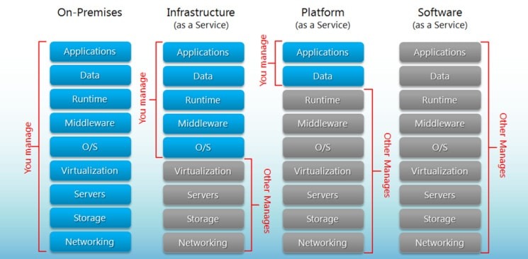
Serverless computing
Focuses on building apps without spending time managing servers/infrastructure.
Feature automatic scaling, built-in high availability, and pay-per-use.
Use of resources when a specific function or event occurs.
Cloud providers handle the deployment, and capacity, and manage the servers.
Example: AWS Lambda, AWS Step Functions.
Easy way to remember SaaS, PaaS, IaaS
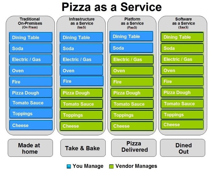
bigcommerce.com
[Avg. reading time: 5 minutes]
Challenges of Cloud Computing
Privacy: “Both traditional and Big Data sets often contain sensitive information, such as addresses, credit card details, or social security numbers.”
So, it’s the responsibility of users to ensure proper security methods are followed.
Compliance: Cloud providers replicate data across regions to ensure safety. If companies have regulations that data should not be stored outside their organization or should not be stored in a specific part of the world.
Data Availability: Everything is dependent on the Internet and speed. It is also dependent on the choice of the cloud provider. Big companies like AWS / GCP / Azure have more data centers and backup facilities.
Connectivity: Internet availability + speed.
Vendor lock-in: Once an organization has migrated its data and applications to the cloud, switching to a different provider can be difficult and expensive. This is known as vendor lock-in. Some cloud agnostic tools like Databricks help enterprises to mitigate this problem, but still, its a challenge.
Cost: Cloud computing can be a cost-effective way to deploy and manage IT resources. However, it is essential to carefully consider your needs and budget before choosing a cloud provider.
Continuous Training: Employees may need to be trained to use cloud-based applications. This can be a cost and time investment.
Constant Change in Technology: Cloud providers constantly improve or change their technology. Recently, Microsoft decided to decommission Synapse and launch a new tool called Fabric.
[Avg. reading time: 4 minutes]
AWS
Terms to Know
Elasticity The ability to acquire resources as you need them and release resources when you no longer need them.
Scale Up vs. Scale Down
Scale-Out vs. Scale In
Latency
Typically latency is a measurement of a round-trip between two systems, such as how long it takes data to make its way between two.
Root User
Owner of the AWS account.
IAM
Identity Access Management
ARN
Amazon Resource Name
For example
arn:aws:iam::123456789012:user/Development/product_1234/*
Policy
Rules
AWS Popular Services
Amazon EC2
Allows you to deploy virtual servers within your AWS environment.
Amazon S3
A fully managed, object-based storage service that is highly available, highly durable, cost-effective, and widely accessible.
AWS IAM (Identify and Access Mgt)
Used to manage permissions to your AWS resources
AWS Management Services
Amazon CloudWatch
A comprehensive monitoring tool allows you to monitor your services and applications in the cloud.
Billing & Budgeting
Helps control the cost.
[Avg. reading time: 6 minutes]
AWS Global Infrastructure
The Primary two items are given below.
- Availability Zones
- Regions
Availability Zones (AZs)
AZs are the physical data centers of AWS.
This is where the actual computing, storage, network, and database resources are hosted that we as consumers, provision within our Virtual Private Clouds (VPCs).
A common misconception is that a single availability zone equals a single data center. Multiple data centers located closely form a single availability zone.
Each AZ will have another AZ in the same geographical area. Each AZ will be isolated from others using a separate power/network like DR.
Many AWS services use low latency links between AZs to replicate data for high availability and resilience purposes.
Multiple AZs are defined as an AWS Regions. (Example: Virginia)
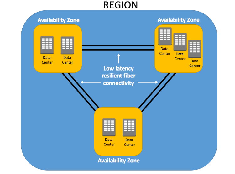
Regions
Every Region will act independently of the others, containing at least two Availability Zones.
Interestingly, only some AWS services are available in some regions.
- US East (N. Virginia) us-east-1
- US East (Ohio) us-east-2
- EU (Ireland) eu-west-1
- EU (Frankfurt) eu-central-1
Note: As of today, AWS is available in 38 regions and 120 AZs
Edge Location
A smaller AWS data center used by Amazon CloudFront and Lambda@Edge to cache content closer to users.
Reduces latency and improves performance for end users, especially for content delivery and inference endpoints.
A user in Singapore fetching from a U.S. model endpoint may hit an Edge Location nearby for lower latency.
Use Cases:
- DNS Resolution (Route 53)
- Content Caching
#aws #region #az #edgelocation
[Avg. reading time: 3 minutes]
CIDR
CIDR = Classless Inter-Domain Routing
It defines how many IP addresses are in a network (or subnet) using a “slash” notation.
Example: 192.168.10.0/24
- Network address: 192.168.10.0
- Prefix Length: /24 means this network will have 256 total IPs
Number of IPs = 2^(32 - prefix)
But AWS and most networks reserve 5 IPs in each subnet:
- 1 for network address
- 1 for broadcast address
- 3 reserved by AWS (for internal routing, DNS, etc.)
/24 subnet gives 251 usable IPs
| CIDR | Subnet Mask | Total IPs | Usable in AWS | Typical Use |
|---|---|---|---|---|
/16 | 255.255.0.0 | 65,536 | 65,531 | Entire VPC range |
/20 | 255.255.240.0 | 4,096 | 4,091 | Large subnet |
/24 | 255.255.255.0 | 256 | 251 | Typical small subnet |
/28 | 255.255.255.240 | 16 | 11 | Small test subnet |
/32 | 255.255.255.255 | 1 | 0 | Single host route |
192.168.10.0 = 11000000.10101000.00001010.00000000
Last 8 digits goes like this
00000100
00000101
00000101
00000110
.....
.....
11111111
[Avg. reading time: 6 minutes]
EC2
(Elastic Cloud Compute)
Compute: Closely related to CPU/RAM
Elastic Compute Cloud (EC2): AWS EC2 provides resizable compute capacity in the cloud, allowing you to run virtual servers as per your needs.
Instance Types: EC2 offers various instance types optimized for different use cases, such as general purpose, compute-optimized, memory-optimized, and GPU instances.
Pricing Models
On-Demand: Pay for computing capacity by the hour or second.
Reserved: Commit to a one or 3-year term and get a discount.
Spot: Bid for unused EC2 capacity at a reduced cost.
Savings Plans: Commit to consistent compute usage for lower prices. AMI (Amazon Machine Image): Pre-configured templates for your EC2 instances, including the operating system, application server, and applications.
Security
Security Groups: Act as a virtual firewall for your instances to control inbound and outbound traffic.
Key Pairs: These are used to access your EC2 instances via SSH or RDP securely.
Elastic IPs: These are static IP addresses that can be associated with EC2 instances. They are useful for hosting services that require a consistent IP.
Auto Scaling: Automatically adjusts the number of EC2 instances in response to changing demand, ensuring you only pay for what you need.
Elastic Load Balancing (ELB): Distributes incoming traffic across multiple EC2 instances, improving fault tolerance and availability.
EBS (Elastic Block Store): Provides persistent block storage volumes for EC2 instances, allowing data to be stored even after an instance is terminated.
Regions and Availability Zones: EC2 instances can be deployed in various geographic regions, each with multiple availability zones for high availability and fault tolerance.
Storage
Persistent Storage
- Elastic Block Storage (EBS) Volumes / Logically attached via AWS network.
- Automatically replicated.
- Encryption is available.
Ephemeral Storage - Local storage
- Physically attached to the underlying host.
- When the instance is stopped or terminated, all the data is lost.
- Rebooting will keep the data intact.
DEMO - Deploy EC2
[Avg. reading time: 19 minutes]
S3
(Simple Storage Service)
It’s an IaaS service. S3 uses Object storage instead of File storage (like your machine or Google Drive)
Warehouse vs Book Shelf
| Scenario | File Storage | Object Storage (S3, Blob) |
|---|---|---|
| Read one small file | Faster (local I/O) | Slight overhead (API call) |
| Read 10,000 files concurrently | Struggles with locks & hierarchy | Scales linearly via APIs |
| Edit file in place | Easy | Not possible (must re-upload) |
| Integrate with Spark / Databricks | Not scalable | Native integration (spark.read.parquet("s3://...")) |
| Network access | Typically mounted | Always network-based (HTTP) |
- Highly Available
- Durable
- Cost Effective
- Widely Accessible
- Uptime of 99.99%
-
Objects and Buckets: The fundamental elements of Amazon S3 are objects and buckets. Objects are the individual data pieces stored in Amazon S3, while buckets are containers for these objects. An object consists of a file and, optionally, any metadata that describes that file.
-
It’s also a regional service, meaning that when you create a bucket, you specify a region, and all objects are stored there.
-
Globally Unique: The name of an Amazon S3 bucket must be unique across all of Amazon S3, that is, across all AWS customers. It’s like a domain name.
-
Globally Accessible: Even though you specify a particular region when you create a bucket, once the bucket is created, you can access it from anywhere in the world using the appropriate URL.
-
-
Scalability: Amazon S3 can scale in terms of storage, request rate, and users to support unlimited web-scale applications.
-
Security: Amazon S3 includes several robust security features, such as encryption for data at rest and in transit, access controls like Identity and Access Management (IAM) policies, bucket policies, and Access Control Lists (ACLs), and features for monitoring and logging activity, like AWS CloudTrail.
-
Data transfer: Amazon S3 supports transfer acceleration, which speeds up uploads and downloads of large objects.
-
Event Notification: S3 can notify you of specific events in your bucket. For instance, you could set up a notification to alert you when an object is deleted from your bucket.
-
Management Features: S3 has a suite of features to help manage your data, including lifecycle management, which allows you to define rules for moving or expiring objects, versioning to keep multiple versions of an object in the same bucket, and analytics for understanding and optimizing storage costs.
-
Consistency: Amazon S3 provides read-after-write consistency for PUTS of new objects and eventual consistency for overwrite PUTS and DELETES.
-
Read-after-write Consistency for PUTS of New Objects: When a new object is uploaded (PUT) into an Amazon S3 bucket, it’s immediately accessible for read (GET) operations. This is known as read-after-write consistency. You can immediately retrieve a new object as soon as you create it. This applies across all regions in AWS, and it’s crucial when immediate, accurate data retrieval is required.
-
Eventual Consistency for Overwrite PUTS and DELETES: Overwrite PUTS and DELETES refer to operations where an existing object is updated (an overwrite PUT) or removed (a DELETE). For these operations, Amazon S3 provides eventual consistency. If you update or delete an object and immediately attempt to read or delete it, you might still get the old version or find it there (in the case of a DELETE) for a short period. This state of affairs is temporary, and shortly after the update or deletion, you’ll see the new version or find the object gone, as expected.
-
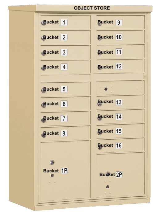
Src: Mailbox
-
S3 is like a building full of mailboxes (buckets). Each bucket has a unique name globally, and you can only access the ones you have keys for (permissions).
-
The overall S3 service is like a large building that contains multiple lockers.
-
Each bucket is a unique container that stores your objects (files, images, datasets).
-
Only authorized users (via IAM roles or bucket policies) can open that specific locker.
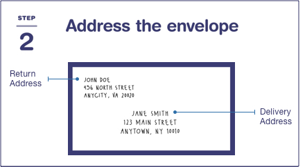
Src: USPS
-
This is the destination — it tells S3 where to deliver or find the object (s3://my-bucket/path/to/file.csv).
-
The envelope is the actual content.
-
Labels on envelope is the object metadata (content-type, size, date and so on)
Notes
Data is stored as an “Object.”
Object storage, also known as object-based storage, manages data as objects. Each object includes the data, associated metadata, and a globally unique identifier.
Unlike file storage, there are no folders or directories in object storage. Instead, objects are organized into a flat address space, called a bucket in Amazon S3’s terminology.
The unique identifier allows an object to be retrieved without needing to know the physical location of the data. Metadata can be customized, making object storage incredibly flexible.
Every object gets a UID (universal ID) and associated META data.
No Folders / SubFolders
For example, if you have an object with the key images/summer/beach.png in your bucket, Amazon S3 has no internal concept of the images or summer as separate entities—it simply sees the entire string images/summer/beach.png as the key for that object.
To store objects in S3, you must first define and create a bucket.
You can think of a bucket as a container for your data.
This bucket name must be unique, not just within the region you specify, but globally against all other S3 buckets, of which there are many millions.
Any object uploaded to your buckets is given a unique object key to identify it.
- S3 bucket ownership is not transferable.
- S3 bucket names should start with alphabets, and - is allowed in between.
- An AWS account can have a maximum of 100 buckets.
More details
#aws #s3 #storage #objectstorage
[Avg. reading time: 6 minutes]
description: Identity Access Management
IAM
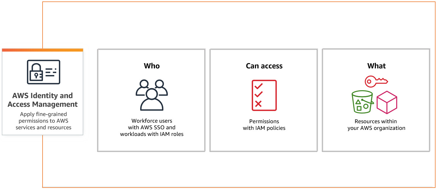
src: Aws
ARN: Amazon Resource Name
Users - Individual Person / Application
Groups - Collection of IAM Users
Policies - Policy sets permission/control access to AWS resources. Policies are stored in AWS as JSON documents.
A Policy can be attached to multiple entities (users, groups, and roles) in your AWS account.
Multiple Policies can be created and attached to the user.
Roles - Set of permissions that define what actions are allowed and denied by an entity in the AWS console. Similar to a user, it can be accessed by any type of entity.
// Examples of ARNs

arn:aws:s3:::my_corporate_bucket/*

arn:aws:s3:::my_corporate_bucket/Development/*

arn:aws:iam::123456789012:user/chandr34

arn:aws:iam::123456789012:group/bigdataclass

arn:aws:iam::123456789012:group/*
Types of Policies
Identity-based policies: Identity-based policies are attached to an IAM user, group, or role (identities). These policies control what actions an identity can perform, on which resources, and under what conditions.
Resource-based policies: Resource-based policies are attached to a resource such as an Amazon S3 bucket. These policies control what actions a specified principal can perform on that resource and under what conditions.
Permission Boundary: You can use an AWS-managed policy or a customer-managed policy to set the boundary for an IAM entity (user or role). A permissions boundary is an advanced feature for using a managed policy to set the maximum permissions that an identity-based policy can grant to an IAM entity.
Inline Policies: Policies that are embedded in an IAM identity. Inline policies maintain a strict one-to-one relationship between a policy and an identity. They are deleted when you delete the identity.
[Avg. reading time: 13 minutes]
AWS CloudShell
AWS CloudShell is a browser-based shell environment available directly through the AWS Management Console. It provides a command-line interface (CLI) to manage and interact with AWS resources securely without needing to install any software or set up credentials on your local machine.
Use Cases
Quick Access to AWS CLI
Allows you to run AWS CLI commands directly without configuring your local machine. It’s perfect for quick tasks like managing AWS resources (e.g., EC2 instances, S3 buckets, or Lambda functions).
Development and Automation
You can write and execute scripts using common programming languages like Python and Shell. It’s great for testing and automating tasks directly within your AWS environment.
Secure and Pre-Configured Environment
AWS CloudShell comes pre-configured with AWS CLI, Python, Node.js, and other essential tools. It uses your IAM permissions, so you don’t need to handle keys or credentials directly, making it secure and convenient.
Access to Filesystem and Persistent Storage
You get a persistent 1 GB home directory per region to store scripts, logs, or other files between sessions, which can be used to manage files related to your AWS resources.
Cross-Region Management
You can access and manage resources across different AWS regions directly from CloudShell, making it useful for multi-region setups.
Basic Commands
    aws s3 ls
    aws ec2 describe-instances

    sudo apt install jq
list_buckets.sh
#!/bin/bash
echo "Listing all S3 buckets:"
aws s3 ls
bash list_buckets.sh
# get account details

aws sts get-caller-identity

# list available regions

aws ec2 describe-regions --query "Regions[].RegionName" --output table

# create a bucket

aws s3 mb s3://chandr34-newbucket

# upload a file to a bucket

echo "Hello, CloudShell!" > hello.txt
aws s3 cp hello.txt s3://chandr34-newbucket

# List files in bucket

aws s3 ls s3://chandr34-newbucket/

# Delete bucket  with files

aws s3 rb s3://chandr34-newbucket --force

# List AMIs

aws ec2 describe-images --owners amazon --query 'Images[*].{ID:ImageId,Name:Name}' --output table

# quickly launch a ec2

aws ec2 create-key-pair --key-name gcnewkeypair --query 'KeyMaterial' --output text > myNewKeyPair.pem

# Change Permission

chmod 0400 myNewKeyPair.pem

# Launch new EC2

aws ec2 run-instances --image-id ami-0866a3c8686eaeeba --count 1 --instance-type t2.micro --key-name gcnewkeypair --security-groups default

# Get Public IP

aws ec2 describe-instances --query "Reservations[].Instances[].PublicIpAddress" --output text

# Login to server

ssh -i myKeyNewPair.pem ubuntu@<getthehostip>

# terminate the instance

aws ec2 terminate-instances --instance-ids <>
Cloud Formation
my-webserver.yml
AWSTemplateFormatVersion: '2010-09-09'
Description: CloudFormation template to launch an Amazon Linux EC2 instance with Nginx installed.

Resources:
  MyEC2Instance:
    Type: AWS::EC2::Instance
    Properties:
      InstanceType: t2.micro
      ImageId: ami-0866a3c8686eaeeba
      KeyName: gcnewkeypair
      SecurityGroupIds:
        - !Ref InstanceSecurityGroup
      UserData:
        Fn::Base64:
          !Sub |
            #!/bin/bash
            apt update -y
            apt install -y nginx
            systemctl start nginx
            systemctl enable nginx
      Tags:
        - Key: Name
          Value: MyNginxServer

  InstanceSecurityGroup:
    Type: AWS::EC2::SecurityGroup
    Properties:
      GroupDescription: Enable SSH and HTTP access
      SecurityGroupIngress:
        - IpProtocol: tcp
          FromPort: 22
          ToPort: 22
          CidrIp: 0.0.0.0/0  # SSH access, restrict this to your IP range for security
        - IpProtocol: tcp
          FromPort: 80
          ToPort: 80
          FromPort: 443
          ToPort: 443
          CidrIp: 0.0.0.0/0  # HTTP access for Nginx

Outputs:
  InstanceId:
    Description: The Instance ID of the EC2 instance
    Value: !Ref MyEC2Instance
  PublicIP:
    Description: The Public IP address of the EC2 instance
    Value: !GetAtt MyEC2Instance.PublicIp
  WebURL:
    Description: URL to access the Nginx web server
    Value: !Sub "http://${MyEC2Instance.PublicIp}"
Launch the Stack via CloudShell
# Create the stack
aws cloudformation create-stack --stack-name gc-stack --template-body file://my-webserver.yml --capabilities CAPABILITY_NAMED_IAM


# Check the status

aws cloudformation describe-stacks --stack-name gc-stack --query "Stacks[0].StackStatus"


aws cloudformation describe-stacks --stack-name gc-stack --query "Stacks[0].Outputs"

# delete the stack

aws cloudformation delete-stack --stack-name gc-stack


aws cloudformation describe-stacks --stack-name gc-stack --query "Stacks[0].StackStatus"

# confirm the deletion status

aws cloudformation list-stacks --query "StackSummaries[?StackName=='gc-stack'].StackStatus"
[Avg. reading time: 16 minutes]
Terraform
Features of Terraform
Infrastructure as Code: Terraform allows you to write, plan, and create infrastructure using configuration files. This makes infrastructure management automated, consistent, and easy to collaborate on.
Multi-Cloud Support: Terraform supports many cloud providers and on-premises environments, allowing you to manage resources across different platforms seamlessly.
State Management: Terraform keeps track of the current state of your infrastructure in a state file. This enables you to manage changes, plan updates, and maintain consistency in your infrastructure.
Resource Graph: Terraform builds a resource dependency graph that helps in efficiently creating or modifying resources in parallel, speeding up the provisioning process and ensuring dependencies are handled correctly.
Immutable Infrastructure: Terraform promotes the practice of immutable infrastructure, meaning that resources are replaced rather than updated directly. This ensures consistency and reduces configuration drift.
Execution Plan: Terraform provides an execution plan (terraform plan) that previews changes before they are applied, allowing you to understand and validate the impact of changes before implementing them.
Modules: Terraform supports reusability through modules, which are self-contained, reusable pieces of configuration that help you maintain best practices and reduce redundancy in your infrastructure code.
Community and Ecosystem: Terraform has a large open-source community and many providers and modules available through the Terraform Registry, which makes it easier to get started and integrate with various services.
Use Cases
- Multi-Cloud Provisioning
- Infrastructure Scaling
- Disaster Recovery
- Environment Management
- Compliance & Standardization
- CI/CD Pipelines
- Speed and Simplicity
- Team Collaboration
- Error Reduction
- Enhanced Security
Install Terraform CLI
<a href="https://developer.hashicorp.com/terraform/downloads"" title="" target="_blank">Terraform Download
Terraform Structure
Provider Block: Specifies the cloud provider or service (e.g., AWS, Azure, Google Cloud) that Terraform will interact with.
provider "aws" {
  region = "us-east-1"
}
Resource Block: Defines the resources to be created or managed. A resource can be a server, network, or other infrastructure component.
resource "aws_instance" "example" {
  ami           = "ami-0c55b159cbfafe1f0"
  instance_type = "t2.micro"
}
Data Block: Fetches information about existing resources, often for referencing in resource blocks.
data "aws_ami" "latest" {
  most_recent = true
  owners      = ["amazon"]
}
Variable Block: Declares input variables to make the script flexible and reusable.
variable "instance_type" {
  description = "Type of instance to use"
  type        = string
  default     = "t2.micro"
}
Output Block: Specifies values to be output after the infrastructure is applied, like resource IDs or connection strings.
output "instance_ip" {
  value = aws_instance.example.public_ip
}
Module Block: Used to encapsulate and reuse sets of Terraform resources.
module "vpc" {
  source = "./modules/vpc"
  cidr_block = "10.0.0.0/16"
}
Locals Block: Defines local values that can be reused in the configuration.
locals {
  environment = "production"
  instance_count = 3
}
SET these environment variables.
export AWS_ACCESS_KEY_ID="your-access-key-id"
export AWS_SECRET_ACCESS_KEY="your-secret-access-key"
Simple S3 Bucket
simple_s3_bucket.tf
terraform {
  required_providers {
    aws = {
      source  = "hashicorp/aws"
      version = "~> 5.70.0"
    }
  }

  required_version = ">= 1.2.0"
}

provider "aws" {
  region = "us-east-1"
  profile = "chandr34"
}

resource "aws_s3_bucket" "demo" {
  bucket = "chandr34-my-new-tf-bucket"

  tags = {
    Createdusing = "tf"
    Environment  = "classdemo"
  }
}

output "bucket_name" {
  value = aws_s3_bucket.demo.bucket
}
Create a new folder
Copy the .tf into it
terraform init
terraform validate
terraform plan
terraform apply
terraform destroy
Variable S3 Bucket
variable_bucket.tf
terraform {
  required_providers {
    aws = {
      source  = "hashicorp/aws"
      version = "~> 5.70.0"
    }
  }

  required_version = ">= 1.2.0"
}

provider "aws" {
  region  = "us-east-1"
  profile = "chandr34"
}

variable "bucket_name" {
  description = "The name of the S3 bucket to create"
  type        = string
}

resource "aws_s3_bucket" "demo" {
  bucket = var.bucket_name

  tags = {
    Createdusing = "tf"
    Environment  = "classdemo"
  }
}

output "bucket_name" {
  value = aws_s3_bucket.demo.bucket
}
Create a new folder
Copy the .tf into it
terraform init
terraform validate
terraform plan
terraform apply -var="bucket_name=chandr34-variable-bucket"
terraform destroy -var="bucket_name=chandr34-variable-bucket"
Variable file
Any filename with extension .tfvars
terraform.tfvars
bucket_name = "chandr34-variable-bucket1"
terraform apply -auto-approve
Please make sure AWS Profile is created.
Create Public and Private Keys
Linux / Mac Users
// create private/public key

ssh-keygen -b 2048 -t rsa -f ec2_tf_demo
Windows Users
Open PuttyGen and create a Key
Terraform
- mkdir simple_ec2
- cd tf-aws-ec2-sample
- Create main.tf
// main.tf
#https://registry.terraform.io/providers/hashicorp/aws/latest

terraform {
  required_providers {
    aws = {
      source  = "hashicorp/aws"
      version = "~> 5.70.0"
    }
  }

  required_version = ">= 1.2.0"
}

provider "aws" {
  region  = "us-east-1"
  profile = "chandr34"
}

resource "aws_key_pair" "generated_key" {
  key_name   = "generated-key-pair"
  public_key = tls_private_key.generated_key.public_key_openssh
}

resource "tls_private_key" "generated_key" {
  algorithm = "RSA"
  rsa_bits  = 2048
}

resource "local_file" "private_key_file" {
  content  = tls_private_key.generated_key.private_key_pem
  filename = "${path.module}/generated-key.pem"
}

resource "aws_instance" "ubuntu_ec2" {
  ami           = "ami-00874d747dde814fa"
  instance_type = "t2.micro"
  key_name      = aws_key_pair.generated_key.key_name
  vpc_security_group_ids = [aws_security_group.ec2_security_group.id]

  tags = {
    Name        = "UbuntuInstance"
    Environment = "classdemo"
  }
}

resource "aws_security_group" "ec2_security_group" {
  name        = "ec2_security_group"
  description = "Allow SSH and HTTP access"

  ingress {
    from_port   = 22
    to_port     = 22
    protocol    = "tcp"
    cidr_blocks = ["0.0.0.0/0"]  # Allow SSH from anywhere (use cautiously)
  }

  ingress {
    from_port   = 80
    to_port     = 80
    protocol    = "tcp"
    cidr_blocks = ["0.0.0.0/0"]  # Allow HTTP from anywhere
  }

  egress {
    from_port   = 0
    to_port     = 0
    protocol    = "-1"
    cidr_blocks = ["0.0.0.0/0"]  # Allow all outbound traffic
  }

  tags = {
    Name = "EC2SecurityGroup"
  }
}

output "ec2_instance_public_ip" {
  value = aws_instance.ubuntu_ec2.public_ip
}

output "private_key_pem" {
  value     = tls_private_key.generated_key.private_key_pem
  sensitive = true
}
goto terminal
- terraform init
- terraform fmt
- terraform validate
- terraform apply
- terraform show
Finally
- terraform destroy
[Avg. reading time: 1 minute]
MLflow Model Lifecycle
[Avg. reading time: 14 minutes]
Decorator
Decorators in Python are a powerful way to modify or extend the behavior of functions or methods without changing their code. Decorators are often used for tasks like logging, authentication, and adding additional functionality to functions. They are denoted by the “@” symbol and are applied above the function they decorate.
def say_hello():
    print("World")

say_hello()
How do we change the output without changing the say hello() function?
wrapper() is not reserved word. It can be anyting.
Use Decorators
# Define a decorator function
def hello_decorator(func):
    def wrapper():
        print("Hello,")
        func()  # Call the original function
    return wrapper

# Use the decorator to modify the behavior of say_hello
@hello_decorator
def say_hello():
    print("World")

# Call the decorated function
say_hello()
When Python sees @decorator_name, it does:
say_hello = hello_decorator(say_hello)
If you want to replace the new line character and the end of the print statement, use end=''
# Define a decorator function
def hello_decorator(func):
    def wrapper():
        print("Hello, ", end='')
        func()  # Call the original function
    return wrapper

# Use the decorator to modify the behavior of say_hello
@hello_decorator
def say_hello():
    print("World")

# Call the decorated function
say_hello()
Multiple functions inside the Decorator
def hello_decorator(func):
    def first_wrapper():
        print("First wrapper, doing something before the second wrapper.")
        #func()

    def second_wrapper():
        print("Second wrapper, doing something before the actual function.")
        #func()

    def main_wrapper():
        first_wrapper()  # Call the first wrapper
        second_wrapper()  # Then call the second wrapper, which calls the actual function
        func()

    return main_wrapper

@hello_decorator
def say_hello():
    print("World")

say_hello()
Multiple Decorators
from functools import wraps
def one(func):
    def one_wrapper():
        print(f"Decorator One: Before function - Called by {func.__name__}")
        func()
        print(f"Decorator One: After function - Called by {func.__name__}")
    return one_wrapper

def two(func):
    def two_wrapper():
        print(f"Decorator Two: Before function - Called by {func.__name__}")
        func()
        print(f"Decorator Two: After function - Called by {func.__name__}")
    return two_wrapper

def three(func):
    def three_wrapper():
        print(f"Decorator Three: Before function - Called by {func.__name__}")
        func()
        print(f"Decorator Three: After function - Called by {func.__name__}")
    return three_wrapper

@one
@two
@three
def say_hello():
    print("Hello, World!")

say_hello()
Decorator Order
one(two(three(say_hello())))

[ONE
    TWO
        THREE
            SAY_HELLO]
Wraps
@wraps is a decorator from Python’s functools module that preserves the original function’s metadata (like its name, docstring, and annotations) when it’s wrapped by another function.
Without using wraps
def some_decorator(func):
    def wrapper():
        """Wrapper docstring"""
        return func()
    return wrapper

@some_decorator
def hello():
    """Original docstring"""
    print("Hi!")

print(hello.__name__)
print(hello.__doc__)
Using Wraps
from functools import wraps

def some_decorator(func):
    @wraps(func)
    def wrapper():
        """Wrapper docstring"""
        return func()
    return wrapper

@some_decorator
def hello():
    """Original docstring"""
    print("Hi!")

print(hello.__name__)
print(hello.__doc__)
Args & Kwargs
*args: This is used to represent positional arguments. It collects all the positional arguments passed to the decorated function as a tuple.**kwargs: This is used to represent keyword arguments. It collects all the keyword arguments (arguments passed with names) as a dictionary.
from functools import wraps

def my_decorator(func):
    @wraps(func)
    def wrapper(*args, **kwargs):
        print("Positional Arguments (*args):", args)
        print("Keyword Arguments (**kwargs):", kwargs)
        result = func(*args, **kwargs)
        return result
    return wrapper

@my_decorator
def example_function(a, b, c=0, d=0):
    print("Function Body:", a, b, c, d)

# Calling the decorated function with different arguments
example_function(1, 2)
example_function(3, 4, c=5)
Popular Example
import time
from functools import wraps

def timer(func):
    @wraps(func)
    def wrapper(*args, **kwargs):
        start = time.time()
        result = func(*args, **kwargs)
        end = time.time()
        print(f"Execution time of {func.__name__}: {end - start} seconds")
        return result
    return wrapper

@timer
def add(x, y):
    """Returns the sum of x and y"""
    return x + y

@timer
def greet(name, message="Hello"):
    """Returns a greeting message with the name"""
    return f"{message}, {name}!"

print(add(2, 3))
print(greet("Rachel"))
The purpose of @wraps is to preserve the metadata of the original function being decorated.
[Avg. reading time: 5 minutes]
HTTP Basics
HTTP (Hypertext Transfer Protocol) is the foundation for data communication on the web.
Common HTTP Methods
| Method | Description | Typical Use |
|---|---|---|
| GET | Retrieve data | Fetch a resource (read-only) |
| POST | Create new data | Add new records or trigger an action |
| PUT | Replace data | Update/replace an existing record |
| DELETE | Remove data | Delete a record |
Popular HTTP Status Codes
200 Series (Success): 200 OK, 201 Created.
300 Series (Redirection): 301 Moved Permanently, 302 Found.
400 Series (Client Error): 400 Bad Request, 401 Unauthorized, 404 Not Found.
500 Series (Server Error): 500 Internal Server Error, 503 Service Unavailable.
REST API
REpresentational State Transfer is a software architectural style developers apply to web APIs.
REST APIs provide simple, uniform interfaces because they can be used to make data, content, algorithms, media, and other digital resources available through web URLs. Essentially, REST APIs are the most common APIs used across the web today.
https://api.zippopotam.us/us/08028

http://api.tvmaze.com/search/shows?q=friends

https://jsonplaceholder.typicode.com/posts

https://jsonplaceholder.typicode.com/posts/1

https://jsonplaceholder.typicode.com/posts/1/comments

https://reqres.in/api/users?page=2

https://reqres.in/api/users/2
CURL & VSCode
curl is a CLI application available for all OS.

https://curl.se/windows/
curl https://api.zippopotam.us/us/08028

curl https://api.zippopotam.us/us/08028 -o zipdata.json
[Avg. reading time: 3 minutes]
Pydantic
Pydantic is a Python library for data validation, type enforcement, and serialization using standard Python type hints.
It ensures the data coming into your app (like API requests, configs, or ML inputs) is valid, typed, and clean — automatically.
Key Features
Automatic validation: Converts and checks input types (e.g., “5” → int(5)).
BaseModel class: Define data schemas by subclassing BaseModel.
Error messages: Tells you exactly which field is invalid and why.
Data parsing: Converts JSON or dicts into Python objects you can use directly.
Integration with FastAPI: FastAPI uses Pydantic models to validate request bodies and auto-generate documentation.
Why It Matters in MLOps
-
Ensures model inputs (e.g., features in an API request) are validated before prediction.
-
Prevents serving errors due to missing or wrong data types.
-
Makes your FastAPI endpoints self-documenting via OpenAPI and /docs.
Example: Google colab
https://colab.research.google.com/drive/1IkROILidYV8iY9HchMGv2EAqQNK5o8d5?usp=sharing
[Avg. reading time: 8 minutes]
Model Flavors
Remember MLflow features (Experiments - Runs - Models - Versions)
Rerun the model again.
git clone https://github.com/gchandra10/uni_multi_model
Popular MLflow Model Flavors
| Flavor | Used For | Typical Libraries / Frameworks |
|---|---|---|
sklearn | Traditional ML models (regression, classification, clustering) | Scikit-Learn, statsmodels |
xgboost | Gradient boosting trees | XGBoost |
lightgbm | High-performance gradient boosting | LightGBM |
catboost | Categorical-feature-friendly boosting | CatBoost |
pytorch | Deep learning and neural networks | PyTorch |
tensorflow / keras | Deep learning models | TensorFlow, Keras |
onnx | Portable models for cross-framework inference | ONNX Runtime |
fastai | Transfer learning and DL pipelines | FastAI |
statsmodels | Statistical / econometric models | statsmodels |
prophet | Time series forecasting | Facebook Prophet |
gluon | Deep learning (MXNet backend) | Apache MXNet |
sparkml | Distributed ML pipelines | Apache Spark MLlib |
pyfunc | Universal interface — wraps all other flavors | MLflow internal meta-flavor |

PyFunc makes ML models cross-platform — one consistent way to load and predict, regardless of how they were built.
-
Just like apps can be built separately for iOS or Android, models in MLflow can be saved in different native formats (like Scikit-Learn, PyTorch, XGBoost, etc.).
-
A cross-platform app works everywhere, and that’s what PyFunc is for ML models: a universal wrapper that runs any model with the same interface.
-
This lets teams serve and reuse models easily, without worrying about which library originally trained them.
For Example:
| Library | Save API | Predict Method |
|---|---|---|
| Scikit-Learn | joblib.dump() | model.predict() |
| TensorFlow | model.save() | model(x) |
| PyTorch | torch.save() | model.forward(x) |
| XGBoost | model.save_model() | model.predict(xgb.DMatrix(x)) |
You can use pyfunc for all the flavors
import mlflow.pyfunc
mlflow.pyfunc.save_model()

---
---
---

model = mlflow.pyfunc.load_model("models:/<name>/<stage>")
model.predict(pd.DataFrame(...))
Advantages
- One simple API for inference. Works the same whether the model was trained in Scikit-Learn, XGBoost, PyTorch, or TensorFlow.
- Reduces code differences between data-science teams using different libraries.
- PyFunc packages the model + environment (conda/requirements) together.
- Guarantees that the model runs identically on local machines, servers, or cloud.
- Ideal for CI/CD pipelines and container builds.
- Can be loaded from: Run path: runs:/<run_id>/model Registry stage: models:/name/Production
- Works seamlessly with MLflow Serving, FastAPI, Docker, or SageMaker deploys.
- Enables easy A/B comparisons between models trained in different frameworks.
- You can subclass mlflow.pyfunc.PythonModel to: Add preprocessing or feature engineering. Postprocess predictions. Integrate external systems (feature store, logging, metrics).
Limitations
- Framework-specific features are lost.
- Input is pandas centric.
- In some cases, can be slower than native runtimes. (Torch/Tensor flow)
https://github.com/gchandra10/uni_multi_model/blob/main/03_load_test_model.py
#pyfunc #mlflow #tensorflow #pytorch
[Avg. reading time: 6 minutes]
Model Serving
mlflow server
Instantly turn a registered model into a REST API endpoint.
Make sure the MLFlow is still running as per the example.
mlflow server --host 127.0.0.1 --port 8080 \
--backend-store-uri sqlite:///mlflow.db
Windows
SET MLFLOW_TRACKING_URI=http://127.0.0.1:8080
MAC/Linux
export MLFLOW_TRACKING_URI=http://127.0.0.1:8080
Serve the Model
mlflow models serve \
  -m "models:/Linear_Regression_Model/1" \
  --host 127.0.0.1 \
  --port 5001 \
  --env-manager local
Use the Model
curl -X POST "http://127.0.0.1:5001/invocations" \
  -H "Content-Type: application/json" \
  --data '{"inputs": [{"ENGINESIZE": 2.0}, {"ENGINESIZE": 3.0}, {"ENGINESIZE": 4.0}]}'
Pros
- Zero-code serving: Just one CLI command — no need to build an API yourself.
- Auto-handles environment: Loads dependencies automatically.
- Ideal for testing and demos.
- Supports model URIs.
Cons
- Single-threaded process.
- Limited customization.
- Minimal built in monitoring.
- Not suited for blue-green / CICD promotion pipelines.
Fast API
-
Modern, high-performance Python web framework for building REST APIs.
-
FastAPI turns Python functions into fully documented, high-performance REST APIs with minimal code.
-
Built on ASGI (Asynchronous Server Gateway Interface) .
-
Designed for speed, type safety, and developer productivity.
Key Features
- Fast execution: Comparable to Node.js & Go — async by design.
- Automatic validation: Uses Pydantic models to validate and parse JSON inputs.
- Auto-generated API docs: Swagger UI available at /docs, ReDoc at /redoc.
- Type hints = API schema: Python typing directly defines request/response schema.
- Easy to test & extend: Works great with Docker, CI/CD, and modern MLOps stacks.
- Supports both sync & async: You can mix blocking ML inference and async endpoints.
export MLFLOW_TRACKING_URI=http://127.0.0.1:8080
Open uni_multi_model in VSCode
cd uni_multi_model
uvicorn fast_app:app --host 127.0.0.1 --port 5002
Uvicorn
- Python runtime Application server used to run Python app code.
- A lightweight, lightning-fast ASGI server (ASGI = Asynchronous Server Gateway Interface).
- Built on uvloop (fast event loop) and httptools (HTTP parser), with native WebSocket support.
- Works great with FastAPI, Pydandic.
#modelserving #mlflow #fastapi
[Avg. reading time: 7 minutes]
Model Serving Types
Model Serving is the process of deploying trained machine-learning models so they can generate predictions on new data.
Once a model is trained and validated, it must be made available to applications, pipelines, or users that need its outputs — whether that’s a batch job scoring millions of records, a web app recommending products, or an IoT stream detecting anomalies.
Model serving sits in the production stage of the MLOps lifecycle, bridging the gap between model development and business consumption.
It ensures models are:
- Accessible (via APIs, pipelines, or streams)
- Scalable (able to handle varying loads)
- Versioned and governed (using registries and lineage)
- Monitored (for drift, latency, and performance)
In modern stacks (e.g., Databricks, AWS SageMaker, GCP Vertex AI), serving integrates tightly with model registries, feature stores, and CI/CD pipelines to enable reliable, repeatable ML deployment.
Batch Model Serving
Batch serving runs inference on large datasets at scheduled intervals (hourly, nightly, weekly).
- Input data is read from storage or database.
- Predictions are generated for all records.
- Outputs are written back to storage or a downstream table.
Example: Predict new car Co2 Emission.
Pros: Efficient, reproducible, simple to schedule. Cons: Not real-time; predictions may get stale.
Demo:
Real-Time (Online) Model Serving
Real-time serving exposes the model as a low-latency API endpoint. Each request is scored on demand and returned within milliseconds to seconds.
How it works:
An application (e.g., web or mobile) calls the API.
The model receives input features and returns a prediction immediately.
As discussed in the previous chapter.
- MlFlow Serving
- FastAPI Serving
Example:
Credit-card fraud detection, dynamic pricing, personalized recommendations.
Pros: Instant feedback, personalized predictions
Cons: Needs always-on infra, online feature store, auto-scaling
Demo
Streaming (Continuous) Model Serving
Streaming serving applies the model continuously to incoming event streams (Kafka, Kinesis, Delta Live Tables).
Instead of single requests, it handles ongoing flows of data.
- Data arrives in small micro-batches or as events.
- The model scores each record as soon as it appears.
- Results are pushed to dashboards, alerts, or storage.
Example:
IoT anomaly detection, clickstream optimization, live sensor analytics.
Pros:
Near real-time, high-throughput, scalable
Cons:
Complex orchestration, harder to monitor and debug.
[Avg. reading time: 7 minutes]
Auto ML
AutoML (Automated Machine Learning) is the process of automating the end-to-end machine-learning workflow, from data preprocessing and model selection to hyperparameter tuning, evaluation, and deployment.
Make machine learning faster, easier, and more accessible, without sacrificing performance.
Instead of a data scientist manually trying dozens of models and tuning parameters, AutoML systems do this automatically, guided by optimization techniques and performance metrics.
- Speeds up experimentation
- Democratizes machine learning
- Improves model quality
- Enables scalable model governance
| Area | Example Use Case | What AutoML Helps With |
|---|---|---|
| Retail | Predict customer churn or recommend products | Automatically build and tune classifiers/regressors |
| Finance | Credit-risk modeling, fraud detection | Feature selection, threshold optimization |
| Healthcare | Predict patient readmission | Imbalanced-data handling, model explainability |
| Energy | Predict CO₂ emissions or fuel consumption | Regression with mixed numeric + categorical inputs |
| Marketing | Forecast campaign ROI | Fast model iteration and ranking |
What AutoML Actually Does
Typical AutoML frameworks automate these stages:
Data Preprocessing
- Missing-value imputation
- Encoding categorical variables
- Normalization or standardization
Feature Engineering
-
Automatic transformations (log, polynomial, interaction terms)
-
Feature selection and importance ranking
Model Selection
- Chooses among algorithms (e.g., Linear, Random Forest, XGBoost, Neural Net)
Model Ensemble / Stacking
- Combines several good models into one stronger ensemble
Model Evaluation and Ranking
- Uses metrics (RMSE, MAE, AUC, F1, etc.) to pick the best
Model Export
- Produces portable artifacts for production (e.g., MOJO, ONNX, pickle)
H2O AutoML
H2O.ai is an open-source AI and machine-learning platform built for speed and scalability.
It’s written in Java and C++ (high performance) with Python and R APIs for easy use.
The flagship open-source library is H2O-3, and H2O AutoML is a major component within it.
Other similar products
- AutoGluon
- Flaml
- PyCaret
- Auto-sklearn
- AutoKeras
Why H2O AutoML Is Popular in Industry
| Feature | Benefit |
|---|---|
| Scalable JVM backend | Runs on a laptop or a multi-node cluster |
| Multiple APIs | Python, R, Java, Scala |
| Easy deployment | Exports MOJO/POJO models for production scoring |
| Interpretable | Provides variable importance and SHAP explanations |
| Open Source | No license barrier; integrates with enterprise tools |
Google Colab
https://colab.research.google.com/drive/1DZjBbcWXeRk-xlmffG7A4zSez7eX1Rba?usp=sharing
[Avg. reading time: 4 minutes]
CPU vs GPU
CPU: few powerful cores optimized for low-latency, branching, and general purpose tasks. Great for data orchestration, preprocessing, control flow.
Use cases in ML:
feature engineering, I/O, tokenization, small classical ML, control logic.
GPU: thousands of simpler cores optimized for massive parallel math, especially dense linear algebra. Great for matrix multiplies, convolutions, attention.
Orders-of-magnitude speedups for medium to large models and batches.
Use cases in ML:
deep learning training, embedding inference, vector search re-ranking, image and generative workloads.
CUDA
GPU is the hardware. CUDA (Compute Unified Device Architecture) is the framework / language and toolkit that unlocks that hardware. Its from nVidia.
When working with GPU, its a must to check whether CUDA is enabled.
There are bunch of GPU’s like Apple Silicon M-Series, Game consoles uses GPU but doesnt have CUDA.
Remember to change the Runtime
https://colab.research.google.com/drive/1byrDchiV4OWdLKOPl8H4UAcdbwFoR7aA?usp=sharing
[Avg. reading time: 0 minutes]
Tools
[Avg. reading time: 6 minutes]
Containers
World before containers
Physical Machines
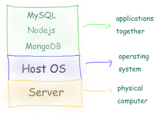
- 1 Physical Server
- 1 Host Machine (say some Linux)
- 3 Applications installed
Limitation:
- Need of physical server.
- Version dependency (Host and related apps)
- Patches ”hopefully” not affecting applications.
- All apps should work with the same Host OS.
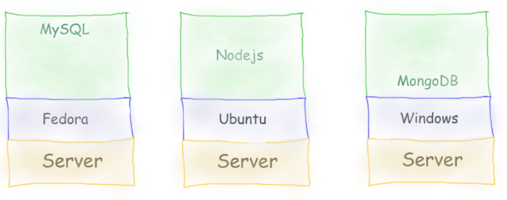
- 3 physical server
- 3 Host Machine (diff OS)
- 3 Applications installed
Limitation:
- Need of physical server(s).
- Version dependency (Host and related apps)
- Patches ”hopefully” not affecting applications.
- Maintenance of 3 machines.
- Network all three so they work together.
Virtual Machines
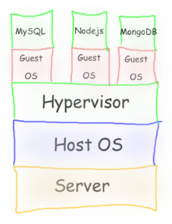
-
Virtual Machines emulate a real computer by virtualizing it to execute applications,running on top of a real computer.
-
To emulate a real computer, virtual machines use a Hypervisor to create a virtual computer.
-
On top of the Hypervisor, we have a Guest OS that is a Virtualized Operating System where we can run isolated applications, called Guest Operating System.
-
Applications that run in Virtual Machines have access to Binaries and Libraries on top of the operating system.
( + ) Full Isolation, Full virtualization ( - ) Too many layers, Heavy-duty servers.
Here comes Containers
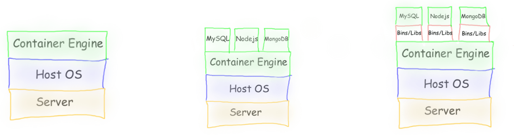
Containers are lightweight, portable environments that package an application with everything it needs to run—like code, runtime, libraries, and system tools—ensuring consistency across different environments. They run on the same operating system kernel and isolate applications from each other, which improves security and makes deployments easier.
-
Containers are isolated processes that share resources with their host and, unlike VMs, don’t virtualize the hardware and don’t need a Guest OS.
-
Containers share resources with other Containers in the same host.
-
This gives more performance than VMs (no separate guest OS).
-
Container Engine in place of Hypervisor.
Pros
- Isolated Process
- Mounted Files
- Lightweight Process
Cons
- Same Host OS
- Security
[Avg. reading time: 6 minutes]
VMs or Containers
VMs are great for running multiple, isolated OS environments on a single hardware platform. They offer strong security isolation and are useful when applications need different OS versions or configurations.
Containers are lightweight and share the host OS kernel, making them faster to start and less resource-intensive. They’re perfect for microservices, CI/CD pipelines, and scalable applications.
Smart engineers focus on the right tool for the job rather than getting caught up in “better or worse” debates.
Use them in combination to make life better.
Popular container technologies
Docker: The most widely used container platform, known for its simplicity, portability, and extensive ecosystem.
Podman: A daemonless container engine that’s compatible with Docker but emphasizes security, running containers as non-root users.
Images
The image is the prototype or skeleton to create a container, like a recipe to make your favorite food.
Container
A container is the environment, up and running and ready for your application.
If Image = Recipe, then Container = Cooked food.
Where to get the Image from?
Docker Hub
For both Podman and Docker, images are from the Docker Hub.
NOTE: INSTALL DOCKER OR PODMAN (Not BOTH)
Podman on Windows
https://podman-desktop.io/docs/installation/windows-install
Once installed, verify the installation by checking the version:
podman info
Podman on MAC
After installing, you need to create and start your first Podman machine:
podman machine init
podman machine start
You can then verify the installation information using:
podman info
Podman on Linux
You can then verify the installation information using:
podman info
Docker Installation
Here is step by step installation
https://docs.docker.com/desktop/setup/install/windows-install/
[Avg. reading time: 0 minutes]
What container does
It brings to us the ability to create applications without worrying about their environment.

[Avg. reading time: 11 minutes]
Container Examples
If you have installed Docker replace podman with docker.
Syntax
docker pull <imagename>
docker run <imagename>
Examples:
docker pull hello-world
docker run hello-world
docker container ls
docker container ls -a
docker image ls
Optional Setting (For PODMAN)
/etc/containers/registries.conf

unqualified-search-registries = ["docker.io"]
Deploy MySQL Database using Containers
Create the following folder
Linux / Mac
mkdir -p container/mysql
cd container/mysql
Windows
md container
cd container
md mysql
cd mysql
Note: If you already have MySQL Server installed in your machine then please change the port to 3307 as given below.
-p 3307:3306 \
Run the container
docker run --name mysql -d \
    -p 3306:3306 \
    -e MYSQL_ROOT_PASSWORD=root-pwd \
    -e MYSQL_ROOT_HOST="%" \
    -e MYSQL_DATABASE=mydb \
    -e MYSQL_USER=remote_user \
    -e MYSQL_PASSWORD=remote_user-pwd \
    docker.io/library/mysql:8.4.4
-d : detached (background mode)
-p : 3306:3306 maps mysql default port 3306 to host machines port 3306
    3307:3306 maps mysql default port 3306 to host machines port 3307

-e MYSQL_ROOT_HOST="%" Allows to login to MySQL using MySQL Workbench
Login to MySQL Container
docker exec -it mysql bash
List all the Containers
docker container ls -a
Stop MySQL Container
docker stop mysql
Delete the container**
docker rm mysql
Preserve the Data for future**
Inside container/mysql
mkdir data
docker run --name mysql -d \
    -p 3306:3306 \
    -e MYSQL_ROOT_PASSWORD=root-pwd \
    -e MYSQL_ROOT_HOST="%" \
    -e MYSQL_DATABASE=mydb \
    -e MYSQL_USER=remote_user \
    -e MYSQL_PASSWORD=remote_user-pwd \
    -v ./data:/var/lib/mysql \
    docker.io/library/mysql:8.4.4
-- Create database
CREATE DATABASE IF NOT EXISTS friends_tv_show;
USE friends_tv_show;

-- Create Characters table
CREATE TABLE characters (
    character_id INT AUTO_INCREMENT PRIMARY KEY,
    first_name VARCHAR(50) NOT NULL,
    last_name VARCHAR(50) NOT NULL,
    actor_name VARCHAR(100) NOT NULL,
    date_of_birth DATE,
    occupation VARCHAR(100),
    apartment_number VARCHAR(10)
);

INSERT INTO characters (first_name, last_name, actor_name, date_of_birth, occupation, apartment_number) VALUES
('Ross', 'Geller', 'David Schwimmer', '1967-10-02', 'Paleontologist', '3B'),
('Rachel', 'Green', 'Jennifer Aniston', '1969-02-11', 'Fashion Executive', '20'),
('Chandler', 'Bing', 'Matthew Perry', '1969-08-19', 'IT Procurement Manager', '19'),
('Monica', 'Geller', 'Courteney Cox', '1964-06-15', 'Chef', '20'),
('Joey', 'Tribbiani', 'Matt LeBlanc', '1967-07-25', 'Actor', '19'),
('Phoebe', 'Buffay', 'Lisa Kudrow', '1963-07-30', 'Massage Therapist/Musician', NULL);

select * from characters;
Build your own Image
mkdir -p container
cd container
Python Example
Follow the README.md
Fork & Clone
git clone https://github.com/gchandra10/docker_mycalc_demo.git
Web App Demo
Fork & Clone
git clone https://github.com/gchandra10/docker_webapp_demo.git
Publish Image to Docker Hub
Login to Docker Hub
- Create a Repository “my_faker_calc”
- Under Account Settings
- Personal Access Token
- Create a PAT token with Read/Write access for 1 day
Replace gchandra10 with yours.
docker login docker.io

enter userid
enter PAT token
Then build the Image with your userid
docker build -t gchandra10/my_faker_calc:1.0  .
docker image ls
Copy the ImageID of gchandra10/my_fake_calc:1.0
Tag the ImageID with necessary version and latest
docker image tag <image_id> gchandra10/my_faker_calc:latest
Push the Images to Docker Hub (version and latest)
docker push gchandra10/my_faker_calc:1.0
docker push gchandra10/my_faker_calc:latest
Image Security
Open Source tool Trivy
https://trivy.dev/latest/getting-started/installation/
trivy image python:3.9-slim

trivy image gchandra10/my_faker_calc

trivy image gchandra10/my_faker_calc --severity CRITICAL,HIGH --format table

trivy image gchandra10/my_faker_calc --severity CRITICAL,HIGH  --output result.txt
[Avg. reading time: 0 minutes]
Productionizing ML Models
- Observability
- Drift
- Security
- Validation Frameworks
- Model Compression
- Ollama
- Best Practices
- SAAS Tools
[Avg. reading time: 3 minutes]
Observability
ML observability means:
- monitoring model behavior
- understanding WHY the model behaves that way
- detecting issues early
- supporting debugging and retraining decisions
ML Observability Pillars
- Data Quality Monitoring
- Drift Monitoring
- Operational / System Monitoring
- Explainability & Bias Monitoring
- Governance, Lineage & Reproducibility
Data Quality Monitoring
Tracks whether the input data is valid, clean, and reliable.
- missing values
- invalid values
- type issues
- schema changes
- outliers
- range violations
- feature null spikes
Operational / System Monitoring
- throughput
- hardware utilization
- inference failures
- API timeouts
- memory leaks
- GPU/CPU load spikes
- queue lag in streaming pipelines
This ensures the model endpoint or batch job is healthy.
Governance, Lineage & Reproducibility
Tracks the lifecycle and accountability of all ML assets.
- dataset versioning
- model versioning
- feature lineage
- pipeline lineage
- audit logs (who deployed, who retrained)
- model approval workflow
- reproducible experiments
- rollback support
[Avg. reading time: 8 minutes]
Drift
Monitoring and observability in ML is about continuously checking:
- What data is coming in
- How that data is changing
- Whether the model’s predictions are still reliable
- Whether the business metrics are degrading
Three key issues:
Data Drift: Incoming feature distributions shift from what the model was trained on.
Concept Drift: The relationship between features and target changes.
Model Performance Decay: Accuracy, precision, recall, RMSE, etc. degrade over time.
Use cases
- Fraud models stop detecting new fraud patterns.
- Demand forecasting fails when consumer behavior changes.
- Recommendation systems decay as user preferences evolve.
- Healthcare/diagnosis models degrade with new demographics.
- NLP sentiment models break due to new slang or cultural shifts.
Example
Phase 1: Training distribution
- sqft mean ~1500
- bedrooms mostly 2 or 3
- house_age mostly 5–15 years
Model learns reasonable patterns.
Phase 2: Production year later
Neighborhood changes + new houses get built.
1. Data Drift
Example:
- sqft mean shifts from 1500 to 2300
- more 4-bedroom homes appear
- house_age shifts from 10 years old to 2 years old (new constructions)
This is feature distribution drift. Model still predicts, but sees very different patterns than training.
2. Concept Drift
Originally:
- Price increases roughly 150 per extra sqft
After market shift:
- Price increases 250 per extra sqft
Meaning: the mapping from features to target changed, even though features look similar.
3. Model Performance Decay
You track weekly RMSE:
- Week 1: RMSE 19k
- Week 15: RMSE 25k
- Week 32: RMSE 42k
Why does it decay?
- Market changed
- New developers building larger homes
- New inflation conditions
- Seasonal patterns changed
- The model is outdated.
Data Quality Drift
Quality of incoming data begins to degrade:
- more missing values
- more zeros
- more invalid/out-of-range values
- more outliers
- schema changes
- feature suddenly becomes constant
- new categories never seen before
This is one of the most important practical drifts.
Example:
“furnished”, “semi-furnished” → suddenly “fully-furnished” appears (NEW category)
Data Freshness Drift (Latency Drift)
Data arrives:
- late
- too early
- stale
- out-of-order
Feature Importance Drift
Rank of feature importance changes:
Example:
- bedrooms used to be the strongest feature
- now open backyard becomes dominant
- previously irrelevant features become important and vice-versa
Input Volume Drift
Sudden spikes or drops in data volume.
Example:
Daily 500 requests suddenly becomes 10,000.
This affects latency, performance, and reliability.
Demo
https://colab.research.google.com/drive/1gf2Qs3avNej6JP-LmKHe022HUiSqbCmy?usp=sharing
git clone https://github.com/gchandra10/python_model_drift
Open Source Tools
https://github.com/evidentlyai/evidently
[Avg. reading time: 9 minutes]
Security
Machine learning systems introduce a whole new attack surface. In traditional software, you secure code, networks, data, and deployments. In ML, you also have to secure training data, model artifacts, feature pipelines, model endpoints, and the feedback loops that continuously update the model.
If ML security is ignored, attackers can quietly poison training data, steal the model, extract sensitive information, or manipulate predictions in production. The impact can be severe: compliance violations, financial loss, biased decisions, or complete system compromise.
Why It Matters
- ML models behave exactly the way the data teaches them. If attackers can tamper with data, you lose trust in the entire pipeline.
- Models deployed as APIs are prime targets for extraction, prompt injections, and inference manipulation.
- Regulatory pressure is rising, and ML systems now need governance similar to financial or healthcare-grade systems.
- Many orgs automate retraining. Without guardrails, an attacker could push poisoned data into the pipeline and silently change model behavior overnight.
1. Data Security
- Validate and sanitize input data before training or inference.
- Detect drift that might be intentional poisoning.
- Maintain lineage: who produced the data, when, from where.
- Encrypt data in transit and at rest.
2. Model Artifact Security
- Store models in a secure registry (MLflow Model Registry or cloud-managed registry).
- Use signed and versioned models to prevent unverified deployments.
- Restrict access at the catalog or registry level using RBAC.
3. Supply Chain Security
- Training code, libraries, dependencies, Docker images, and notebooks can be compromised.
- Use vulnerability scanning tools on Python packages and containers.
- Pin versions using pyproject.toml or UV/Poetry lockfiles.
- Verify model lineage (code version, data version, training environment).
4. API & Endpoint Hardening
- Rate limiting and throttling to prevent model extraction.
- Authentication and authorization around inference endpoints.
- Input validation to avoid adversarial attacks and prompt injections (LLMs).
- Don’t expose internal model metadata via the API.
5. Monitoring & Detection
- Track prediction patterns to catch sudden spikes or targeted manipulation.
- Use model drift & data drift monitoring tools.
- Alert when confidence scores change unpredictably.
- Store logs for forensics.
6. Secrets & Environment Security
- Never hardcode API keys into notebooks or training code.
- Use cloud secret managers or Databricks secret scopes.
- Lock down S3/Blob/GCS buckets and model storage.
- Use network isolation: private endpoints, VPC peering, firewall rules.
How To Ensure Models Are Not Vulnerable
- Implement model reviews as part of CI/CD, including robustness tests.
- Continuously test your data pipelines for poisoning or schema violations.
- Use secure serving infrastructure (no local Flask servers in production).
- Perform penetration testing specifically targeted at model endpoints.
- Automate retraining only when data validation checks pass.
- Track every model version, input source, and deployment environment.
- Keep models and features inside secured catalogs with RBAC and audit logs.
- Use zero-trust principles for every pipeline component.
Popular Tools
FalconPy by Crowdstrike
[Avg. reading time: 5 minutes]
Validation Frameworks
Data validation frameworks help you prove your data is correct before you process or model it.Instead of writing ad-hoc if-else checks, you declare rules once and let the framework enforce them automatically.
- Consistency
- Repeatability
- Cleaner code
- Faster debugging
- Less human error
Validation Frameworks
- Detect bad data early instead of debugging downstream failures
- Enforce rules across teams so everyone validates the same way
- Automate thousands of checks with very little code
- Reduce manual cleanup work that normally takes hours
- Make pipelines safer, more predictable, and easier to maintain
- Shift data quality to where it belongs: before transformation and modeling
| Manual Validation | Framework-Based Validation |
|---|---|
| Lots of custom code | Declare rules once |
| Hard to maintain | Reuse rules everywhere |
| Easy to miss edge cases | Remove 70–90 percent of custom code. |
| Never consistent between developers | Fail fast instead of debugging downstream |
| Repeated onboarding pain | Easier onboarding for new developers and analysts |
Popular Tools
Pandera (Python)
- Easiest for Python pipelines
- Schema-based, great for ML workflows
- Integrates with Pandas, Polars, Dask, Spark
- Treats data validation like unit tests
Pydantic
- Row-level validation
- Excellent for API inputs and ML inference
- Great complement to Pandera, not a dataframe validator
Pydantic + Pandera
- Pydantic is for validating one row at a time.
- Pandera is for validating the whole dataset at once.
- Pydantic shines in ML inference, web APIs, and configuration files.
- Pandera shines in ETL, data cleaning, feature engineering, and ML training pipelines.
git clone https://github.com/gchandra10/python_validator_demo
#pandera #pydantic #validationframework
[Avg. reading time: 5 minutes]
Model Compression
Model compression is the set of techniques used to reduce the size and computational cost of a trained model while keeping its accuracy almost the same.
Why It Exists
- Speed up inference
- Reduce memory footprint
- Fit models on cheaper hardware
- Reduce serving cost
- Enable on-device ML (phones, edge devices, IoT)
- Allow high-traffic systems to scale
Without Compression
- Slow predictions
- GPU or CPU bottlenecks
- More servers needed to keep up
- Higher inference bill
- Some environments can’t run your model at all
- Increased latency kills user experience
Photo Analogy
The popular mechanisms include
- Quantization
Quantization refers to the process of reducing the precision or bit-width of the numerical values used to represent model parameters usually from 𝑛 bits to 𝑚 bits, where 𝑛 > 𝑚.
In ML, FP32 (Floating Point 32 bits) is the default, by quantization method we convert the 32bits to 16 or 8 bits and achieve similar results.
https://colab.research.google.com/drive/1SHGqVZhk8tKpuGQ3KqLhUXIk8NU9W2Er?usp=sharing
When using this with mlflow, log both the models, artifacts and serve the ones depending upon the usecase.
- Distillation
Model distillation, also known as knowledge distillation, is a technique where a smaller model, often referred to as a student model, is trained to mimic the behavior of a larger, more complex model, known as a teacher model. The goal is to transfer the knowledge and performance of the larger model to the smaller one.
Reading whole book vs Nudging with hints and references
#compression #quantization #distillation
[Avg. reading time: 4 minutes]
Ollama
-
Ollama is an open-source tool that allows you to run large language models (LLMs) on your local machine, providing privacy and offline access.
-
It simplifies the process of downloading, running, and managing LLMs with a user-friendly interface, both via a command-line interface (CLI) and an API.
-
It’s designed for developers and researchers who want to customize and experiment with AI models locally, without depending on cloud services.
Install
Download and Install
https://ollama.com/
Open Terminal
ollama

ollama list

ollama pull deepseek-r1:8b

ollama run deepseek-r1:8b
To close the prompt
/bye
Roles
- user: The human asking questions or giving instructions.
- assistant : The model’s response role. This is what the LLM outputs.
- system : Optional. Used to set initial behavior or constraints, similar to system prompts in OpenAI/ChatGPT.
git clone https://github.com/gchandra10/python_ollama_demo.git
chat() - conversational, role-based, template-aware generate() - raw LLM token generation, no chat template, no memory
Build Custom Models
- Create a Modelfile
- Mention the model and prompt
- Create and use the new Model
[Avg. reading time: 6 minutes]
Best Practices
Continuous Integration (CI): Automate testing and validation for code, data, and models before deployment.
Continuous Delivery/Deployment (CD): Automate the deployment of the complete ML pipeline and the trained model to production environments (often using Docker/Kubernetes).
Continuous Training (CT): Implement automated triggers to retrain models based on performance degradation (drift) or arrival of significant new data.
Version Control: Use Git for code and configuration. Crucially, version control datasets (Data Versioning) and model artifacts (Model Registry).
Reproducibility: Log all experiment metadata—including hyperparameters, package dependencies, and data/code versions—to enable exact reproduction of any past result.
Infrastructure as Code (IaC): Manage all compute resources and environments (e.g., training clusters, deployment services) using code (e.g., Terraform) for consistency.
Continuous Monitoring: Track both operational metrics (latency, throughput, resource usage) and model performance metrics (accuracy, precision, business KPIs) in production.
Drift Detection: Actively monitor for Data Drift (input data changes) and Concept Drift (target relationship changes) and set up automated alerts and retraining workflows.
Data Validation: Implement continuous checks on the schema, quality, and statistical properties of input data streams before they reach the model.
Model Governance & Lineage: Maintain a clear audit trail of every model, documenting who trained it, when, and with what specific assets, for regulatory compliance and debugging.
Modular Pipelines: Break the ML workflow (data ingestion, preprocessing, training, evaluation, deployment) into independent, reusable components.
Feature Stores: Use a centralized platform to define, serve, and share reusable features across different models and teams, ensuring consistency between training and serving.
Collaboration: Facilitate smooth handoffs and shared ownership between Data Scientists, ML Engineers, and Operations teams through common tools and standardized interfaces.
[Avg. reading time: 4 minutes]
SAAS Tools for MlFlow
These platforms streamline the entire machine learning lifecycle, often integrating MLflow’s capabilities.
Amazon SageMaker: AWS’s comprehensive, fully-managed platform that covers the entire ML workflow from data preparation to deployment and monitoring.
Google Vertex AI: Google Cloud’s unified platform for building, deploying, and scaling ML models, which includes MLOps tools like pipelines, a model registry, and monitoring.
Microsoft Azure Machine Learning: A cloud service that provides a range of tools and a unified environment to accelerate and manage the ML project lifecycle, with strong native MLflow integration.
Databricks (Managed MLflow): Databricks, co-founded by the creators of MLflow, offers a fully managed and enhanced version of MLflow tightly integrated with their lakehouse platform.
Benefits
Enhanced Collaboration: Provides a shared, centralized platform (via the Tracking Server and Model Registry UI) where data scientists can log, view, compare, and share experiment results and model versions.
Efficient Model Lifecycle Management: The Model Registry offers governance and an audit trail by controlling the transition of model versions through different stages (e.g., from Staging to Production) and linking them to their original training runs.
#saastools #sagemaker #azureml #googlevertexai
[Avg. reading time: 2 minutes]
Good Reads
These are just resources I found interesting and thought you might too. I’m not connected to them and can’t vouch for everything, but I’m sharing in the spirit of helping you discover new ideas, books, and opportunities.
Google Colab Free
https://blog.google/outreach-initiatives/education/colab-higher-education/
DeepLearning.ai
https://www.deeplearning.ai/
Notebook LM
https://notebooklm.google/
ByteByteGo
It’s a very, very useful YT channel.
https://www.youtube.com/@ByteByteGo/videos
Loaded with lots and lots of useful information.
Tags
<abbr title="bidirectional encoder representations from transformers">bert</abbr>
/MLOps & AI Overview/ML Lifecycle/Feature Engineering/Embeddings
agents
/MLOps & AI Overview/AI then and now/Agentic AI
ai-ml
/MLOps & AI Overview/AI then and now/Differences
artificialintelligence
/MLOps & AI Overview/AI then and now
automation
/Developer Tools/JQ
automl
/MLflow Model Lifecycle/Auto ML
aws
/Cloud/AWS/AWS Global Infra
/Cloud/AWS/CloudShell
/Cloud/AWS/EC2
/Cloud/AWS/IAM
/Cloud/AWS/S3
az
/Cloud/AWS/AWS Global Infra
azureml
/Productionizing ML Models/SAAS Tools
batch
/MLflow Model Lifecycle/Model Serving Types
bestpractices
/Productionizing ML Models/Best Practices
challenges
/Cloud/Challenges
cicd
/MLOps & AI Overview/AI then and now/MLOps
cidr
/Cloud/AWS/CIDR
classification
/MLOps & AI Overview/AI then and now/Machine Learning
claude
/MLOps & AI Overview/AI then and now/Generative AI
clean
/MLOps & AI Overview/ML Lifecycle
cleaning
/MLOps & AI Overview/ML Lifecycle/Data Preparation
cli
/Cloud/AWS/CloudShell
/Developer Tools/DuckDB
/Developer Tools/JQ
cloud
/Cloud/Challenges
/Cloud/Overview
/Cloud/Types
cloudshell
/Cloud/AWS/CloudShell
collect
/MLOps & AI Overview/ML Lifecycle
compression
/Productionizing ML Models/Model Compression
container
/Tools/Containers/What container does
containers
/Tools/Containers
cpu
/MLflow Model Lifecycle/CPU vs GPU
data
/MLOps & AI Overview/Introduction
/MLOps & AI Overview/ML Lifecycle/Data Preparation
databricks
datacleaning
/MLOps & AI Overview/ML Lifecycle/Data Cleaning
dataimputation
/MLOps & AI Overview/ML Lifecycle/Data Imputation
datavalidation
/MLflow Model Lifecycle/pydantic
decorator
/MLflow Model Lifecycle/Decorator
densevector
/MLOps & AI Overview/ML Lifecycle/Feature Engineering/Vectors
deserialization
/MLOps & AI Overview/Terms to Know
development
/MLOps & AI Overview/Life Before MLOps
devops
/MLOps & AI Overview/AI then and now/MLOps
disclaimer
distillation
/Productionizing ML Models/Model Compression
docker
/Tools/Containers/Container Examples
/Tools/Containers/VMs or Containers
domain_specific
/MLOps & AI Overview/ML Lifecycle/Feature Engineering
drift
/Productionizing ML Models/Drift
dropdata
/MLOps & AI Overview/ML Lifecycle/Data Imputation
duckdb
/Developer Tools/DuckDB
ec2
/Cloud/AWS/EC2
edgelocation
/Cloud/AWS/AWS Global Infra
embeddeddb
/Developer Tools/SQLite
embeddings
/MLOps & AI Overview/ML Lifecycle/Feature Engineering/Embeddings
encode
/MLOps & AI Overview/ML Lifecycle/Data Imputation
error
/Developer Tools/Error Handling
evaluate
/MLOps & AI Overview/ML Lifecycle
examples
/MLOps & AI Overview/Examples
/Tools/Containers/Container Examples
exception
/Developer Tools/Error Handling
experiment
/MLflow Introduction/MLflow Experiment Structure
expert-systems
/MLOps & AI Overview/AI then and now/Expert Systems
explanation
/MLOps & AI Overview/Model vs Library vs Framework/Explanation
fastapi
/MLflow Model Lifecycle/Model Serving
feature_engineering
/MLOps & AI Overview/ML Lifecycle/Feature Engineering
finance
/MLOps & AI Overview/Examples
framework
/MLOps & AI Overview/Model vs Library vs Framework
fuzziness
/MLOps & AI Overview/AI then and now/Fuzzy Logic
fuzzy-logic
/MLOps & AI Overview/AI then and now/Fuzzy Logic
genai
/MLOps & AI Overview/AI then and now/Differences
generativeai
/MLOps & AI Overview/AI then and now/Generative AI
git
goodreads
googlevertexai
/Productionizing ML Models/SAAS Tools
gpt
/MLOps & AI Overview/AI then and now/Generative AI
gpu
/MLflow Model Lifecycle/CPU vs GPU
healthcare
/MLOps & AI Overview/Examples
http
/MLflow Model Lifecycle/HTTP Basics
iaac
/Cloud/Terraform
iaas
/Cloud/Types
iam
/Cloud/AWS/IAM
ipv4
/Cloud/AWS/CIDR
jobs
/MLOps & AI Overview/Job Opportunities
jq
/Developer Tools/JQ
json
/Developer Tools/JQ
/MLflow Introduction/YAML
knn
/MLOps & AI Overview/ML Lifecycle/Data Imputation
label_encoding
/MLOps & AI Overview/ML Lifecycle/Data Encoding
library
/MLOps & AI Overview/Model vs Library vs Framework
/MLOps & AI Overview/Model vs Library vs Framework/Explanation
linearalgebra
/MLOps & AI Overview/Statistical vs ML Models
lint
/Developer Tools/Other Python Tools
llm
/MLOps & AI Overview/AI then and now/Differences
/Productionizing ML Models/Ollama
localdb
/Developer Tools/SQLite
machinelearning
/MLOps & AI Overview/AI then and now
medallion
/MLOps & AI Overview/AI then and now/MLOps
ml
/MLOps & AI Overview/Statistical vs ML Models
mlcleaning
/MLOps & AI Overview/ML Lifecycle/Data Cleaning
mlengineer
/MLOps & AI Overview/Introduction
/MLOps & AI Overview/Job Opportunities
mlflow
/MLflow Introduction/MLflow Experiment Structure
/MLflow Introduction/MLflow Features
/MLflow Model Lifecycle/Model Flavors
/MLflow Model Lifecycle/Model Serving
mlflow_server
/MLflow Introduction/MLflow Features
mlops
/MLOps & AI Overview/AI then and now/Differences
/MLOps & AI Overview/AI then and now/MLOps
/MLOps & AI Overview/Introduction
/MLOps & AI Overview/Life Before MLOps
/Productionizing ML Models/Best Practices
/Productionizing ML Models/Drift
/Productionizing ML Models/Observability
/Productionizing ML Models/Security
mlopsengineer
/MLOps & AI Overview/Job Opportunities
model
/MLOps & AI Overview/Model vs Library vs Framework
modelserving
/MLflow Model Lifecycle/Model Serving
mse
/MLOps & AI Overview/Model vs Library vs Framework
mypy
/Developer Tools/Other Python Tools
nlp
/MLOps & AI Overview/ML Lifecycle/Feature Engineering/Embeddings
normalize_data
/MLOps & AI Overview/ML Lifecycle/Data Cleaning
objectstorage
/Cloud/AWS/S3
observability
/Productionizing ML Models/Observability
ollama
/Productionizing ML Models/Ollama
onehot_encoding
/MLOps & AI Overview/ML Lifecycle/Data Encoding
overfitting
/MLOps & AI Overview/Terms to Know
overview
/Cloud/Overview
paas
/Cloud/Types
pandera
/Productionizing ML Models/Validation Frameworks
parquet
/Developer Tools/DuckDB
parser
/Developer Tools/JQ
pep
/Developer Tools/Other Python Tools
permissions
/Cloud/AWS/IAM
podman
/Tools/Containers/VMs or Containers
poetry
/Developer Tools/Introduction
production
/MLOps & AI Overview/Life Before MLOps
pydantic
/MLflow Model Lifecycle/pydantic
/Productionizing ML Models/Validation Frameworks
pyfunc
/MLflow Model Lifecycle/Model Flavors
pytest
/Developer Tools/Unit Test
python
/Developer Tools/Introduction
/MLflow Introduction/YAML
/MLflow Model Lifecycle/Decorator
pytorch
/MLflow Model Lifecycle/Model Flavors
quantization
/Productionizing ML Models/Model Compression
r2score
/MLOps & AI Overview/Model vs Library vs Framework
realtime
/MLflow Model Lifecycle/Model Serving Types
region
/Cloud/AWS/AWS Global Infra
regression
/MLOps & AI Overview/AI then and now/Machine Learning
resources
restapi
/MLflow Model Lifecycle/HTTP Basics
retail
/MLOps & AI Overview/Examples
rl
/MLOps & AI Overview/AI then and now/Reinforcement Learning
rlhf
/MLOps & AI Overview/AI then and now/Reinforcement Learning
robotics
/MLOps & AI Overview/AI then and now/Reinforcement Learning
ruff
/Developer Tools/Other Python Tools
rulebased
/MLOps & AI Overview/AI then and now/Expert Systems
run
/MLflow Introduction/MLflow Experiment Structure
rust
/Developer Tools/UV
s3
/Cloud/AWS/S3
saas
/Cloud/Types
saastools
/Productionizing ML Models/SAAS Tools
sagemaker
/Productionizing ML Models/SAAS Tools
security
/Productionizing ML Models/Security
serialization
/MLOps & AI Overview/Terms to Know
server
/Cloud/AWS/EC2
serving
/MLflow Introduction/MLflow Features
singlefiledatabase
/Developer Tools/DuckDB
sparsevector
/MLOps & AI Overview/ML Lifecycle/Feature Engineering/Vectors
sqlite
/Developer Tools/SQLite
statistics
/MLOps & AI Overview/Statistical vs ML Models
storage
/Cloud/AWS/S3
streaming
/MLflow Model Lifecycle/Model Serving Types
subnet
/Cloud/AWS/CIDR
supervised
/MLOps & AI Overview/AI then and now/Machine Learning
/MLOps & AI Overview/Types of ML Models
tabularvector
/MLOps & AI Overview/ML Lifecycle/Feature Engineering/Vectors
target_encoding
/MLOps & AI Overview/ML Lifecycle/Data Encoding
tensorflow
/MLflow Model Lifecycle/Model Flavors
terraform
/Cloud/Terraform
tools
/Developer Tools/DuckDB
/Developer Tools/JQ
train
/MLOps & AI Overview/ML Lifecycle
try
/Developer Tools/Error Handling
underfitting
/MLOps & AI Overview/Terms to Know
unittesting
/Developer Tools/Unit Test
unsupervised
/MLOps & AI Overview/AI then and now/Machine Learning
/MLOps & AI Overview/Types of ML Models
user
/Cloud/AWS/IAM
uv
/Developer Tools/Introduction
/Developer Tools/UV
validationframework
/Productionizing ML Models/Validation Frameworks
vectors
/MLOps & AI Overview/ML Lifecycle/Feature Engineering/Vectors
venv
/Developer Tools/Introduction
/Developer Tools/UV
vm
/Cloud/AWS/EC2
/Tools/Containers
/Tools/Containers/VMs or Containers
word2vec
/MLOps & AI Overview/ML Lifecycle/Feature Engineering/Embeddings
wraps
/MLflow Model Lifecycle/Decorator
yaml
/MLflow Introduction/YAML